Images of the Russian Empire -- Colorizing the Prokudin-Gorskii Photo Collection
Aligning RGB channels from glass plate negatives and enhancing them for better visual quality
Introduction
Sergei Mikhailovich Prokudin-Gorskii (1863-1944) was a chemist and photographer (his portrait above), best known as a pioneer of color photography. With special permission from the Tzar, he traveled across Russia and neighboring regions carrying a custom-designed camera. Due to the technical limitations of that era, each so-called “color photograph” was actually recorded as three separate negatives on a single specially shaped glass plate, each taken through a red, green, or blue filter. Fortunately, many of these high-quality negatives have been preserved and are now housed at the Library of Congress (LOC), which has digitized and publicly released them. As a result, we have the unique opportunity to glimpse the Russian Empire in color more than a century ago.
In this project, we start from the digitized glass plates provided by the LOC, separate the three RGB channels, and align them to reconstruct plausible color images that Prokudin-Gorskii wanted to share. Different metrics and alignment algorithms are explored to achieve accurate and efficient alignment even for large high-resolution scans. In addition, a series of post-processing enhancement techniques, including automatic cropping, white balance, contrast adjustment, and color remapping, are applied to improve visual quality and produce more natural results.
Highlights
- Exhaustive search for small JPGs using NCC
- Image pyramid for large TIFs for better efficiency
- Robust alignment via Sobel gradient-domain NCC
- Automatic border cropping (edge density + k-part trick)
- Automatic white balance (white patch assumption with tricks)
- Color remapping (linear mapping)
- Automatic contrast adjustment (CLAHE)
Aligning Small JPG Images
Metrics for Image Alignment
Before aligning the images, one needs to define a metric to quantify "how well the images are aligned." This can be achieved through measuring the similarity between two images (patches). With a reference image $P$ and a target image $I$ (that we want to align with $P$), we define a region/patch $N$ that we want to align, then, our goal is to quantify how similar the region $N$ in $I$ is to $P$ after shifting $I$ by $(u,v)$. Two simple metrics are provided:
- Sum of Squared Differences (SSD) :the squared L2 norm between two images in the pixel/feature space,
$$ \text{SSD}(u,v) = \sum_{(x,y)\in N} \left[I(u+x, v+y) - P(x,y)\right]^2 $$
- Normalized Cross-Correlation (NCC): the dot product between two images in the pixel/feature space, i.e., the cosine similarity between two images after subtracting their mean and normalization
$$ \text{NCC}(u,v) = \frac{\sum_{(x,y)\in N}\left[I(u+x,v+y)-\bar I\right]\left[P(x,y)-\bar P\right]} {\sqrt{\sum_{(x,y)\in N}\left[I(u+x,v+y)-\bar I\right]^2}\sqrt{\sum_{(x,y)\in N}\left[P(x,y)-\bar P\right]^2}} $$
With a glance at the definitions above, it is apparent that NCC should behave more robustly than SSD, since it is less sensitive to global shift (via subtracting the mean) and scaling (by normalization), which are both general issues in our case because Prokudin-Gorskii's 3 channels were not taken simultaneously with the same exposure. Therefore, for our implementation, let's start with NCC.
Pre-Processing: Patching
Before applying the alignment algorithm, appropriate pre-processing is required to improve robustness. In particular, computing the similarity metric only on the central region of the image (e.g., the central $90\%$) helps to avoid boundary artifacts. Since metrics like SSD and NCC rely heavily on pixel intensities, including these border regions may significantly degrade their reliability. Therefore, we restrict the calculation to a central patch for more stable scoring.
Search Algorithm: Exhaustive Search
With the similarity metric and the search space (either in the raw pixel space or a transformed feature space) defined, the optimal alignment can be obtained by searching over possible shifts. Here, we adopt a simple exhaustive search in the raw pixel space. The implementation details are as follows:
- Search grid: allow shifts within $[-15, 15]$ pixels around the center $(0, 0)$ in both $x$ and $y$ directions
- Metric: use NCC, which is more robust than SSD as we discussed above.
- Scoring region: restrict metric computation to a central crop, ignoring approximately $10\%$ of the margin to reduce border artifacts
- Output: evaluate all candidate shifts in the grid and return the optimal $(dx, dy)$ for G and R relative to B
Results of Single-Scale Alignment (Exhaustive Search + NCC over Raw Pixel Space on Small JPG Images)
The results are presented below, following the order such that the shift of R channel $(dx, dy)$, shift of G channel $(dx, dy)$, and run time.
_(2, -3)_(0.84).jpg)
R(2, 3) G(2, -3) 0.84s
_(2, 3)_(0.87).jpg)
R(3, 6) G(2, 3) 0.87s
_(2, 5)_(0.83).jpg)
R(3, 12) G(2, 5) 0.83s
Aligning Large TIF Images
Image Pyramid for Faster Alignment
The exhaustive search algorithm works reasonably well for small images with limited search ranges. However, its computational cost grows dramatically with the search window and image resolution, which quickly becomes impractical. For instance, performing the exhaustive search over a shift range of $[-50, 50]$ pixels in both $x$ and $y$ directions on the raw TIF image (without parallelization) may take over 20 minutes!
Therefore, more efficient methods should be considered. Here we implement a coarse-to-fine alignment with image pyramid, where for each level, an exhaustive search is performed, but only within a much smaller local search window.
More specifically, each level is constructed by applying a blur followed by downsampling (by a factor of 2 in our implementation). Blurring is necessary before downsampling at each level, aiming to avoid aliasing. The alignment starts from the coarsest level, and the optimal shift is propagated to the next finer level as the initial guess, until the finest level (the raw image) is reached. Therefore, except for the coarsest level, the searching space at each level is reduced significantly, which is much smaller than the original searching space of naive exhaustive search.
Implementation details include:
- Build pyramids through "blur + downsampling by 2" (via $\texttt{cv2.resize}$ interpolated by $\texttt{INTER_AREA}$), until minimum size (e.g., 300 px).
- Start from the coarsest level with a wide search range (e.g., $[-20, 20]$) around the initial guess (e.g., the center $(0, 0)$), get the optimal shift.
- At finer levels, use the last level's optimal shift (scaled by the downsampling factor, e.g., 2) as the initial guess, then search over a smaller range (e.g., $[-3, 3]$) around it for the new optimal shift.
- Repeat step 3 until the finest level is reached, i.e., the raw image.
Results of Multi-Scale Alignment (Exhaustive Search + NCC over Raw Pixel Space on All Images)
_(2, 5)_(1.52).jpg)
R(3,12) G(2,5) 1.52s
_(-12, 24)_(16.01).jpg)
R(-5,58) G(-12,24) 16.01s
_(24, 49)_(16.40).jpg)
R(55,104) G(24,49) 16.40s
_(16, 60)_(16.39).jpg)
R(14,124) G(16,60) 16.39s
R(23,89) G(17,40) 16.56s
_(21, 38)_(16.58).jpg)
R(35,77) G(21,38) 16.58s
_(-2, -3)_(16.83).jpg)
R(-9,76) G(-2,-3) 16.83s
_(-17, 41)_(16.63).jpg)
R(-29,92) G(-17,41) 16.63s
_(10, 82)_(16.82).jpg)
R(12,178) G(10,82) 16.82s
_(2, -3)_(1.51).jpg)
R(2,3) G(2,-3) 1.51s
_(29, 79)_(17.10).jpg)
R(34,175) G(29,79) 17.10s
_(-7, 49)_(17.23).jpg)
R(-25,96) G(-7,49) 17.23s
_(13, 55)_(16.54).jpg)
R(10,112) G(13,55) 16.54s
_(2, 3)_(1.54).jpg)
R(3,6) G(2,3) 1.54s
Bells & Whistles
Failure Mode Analysis
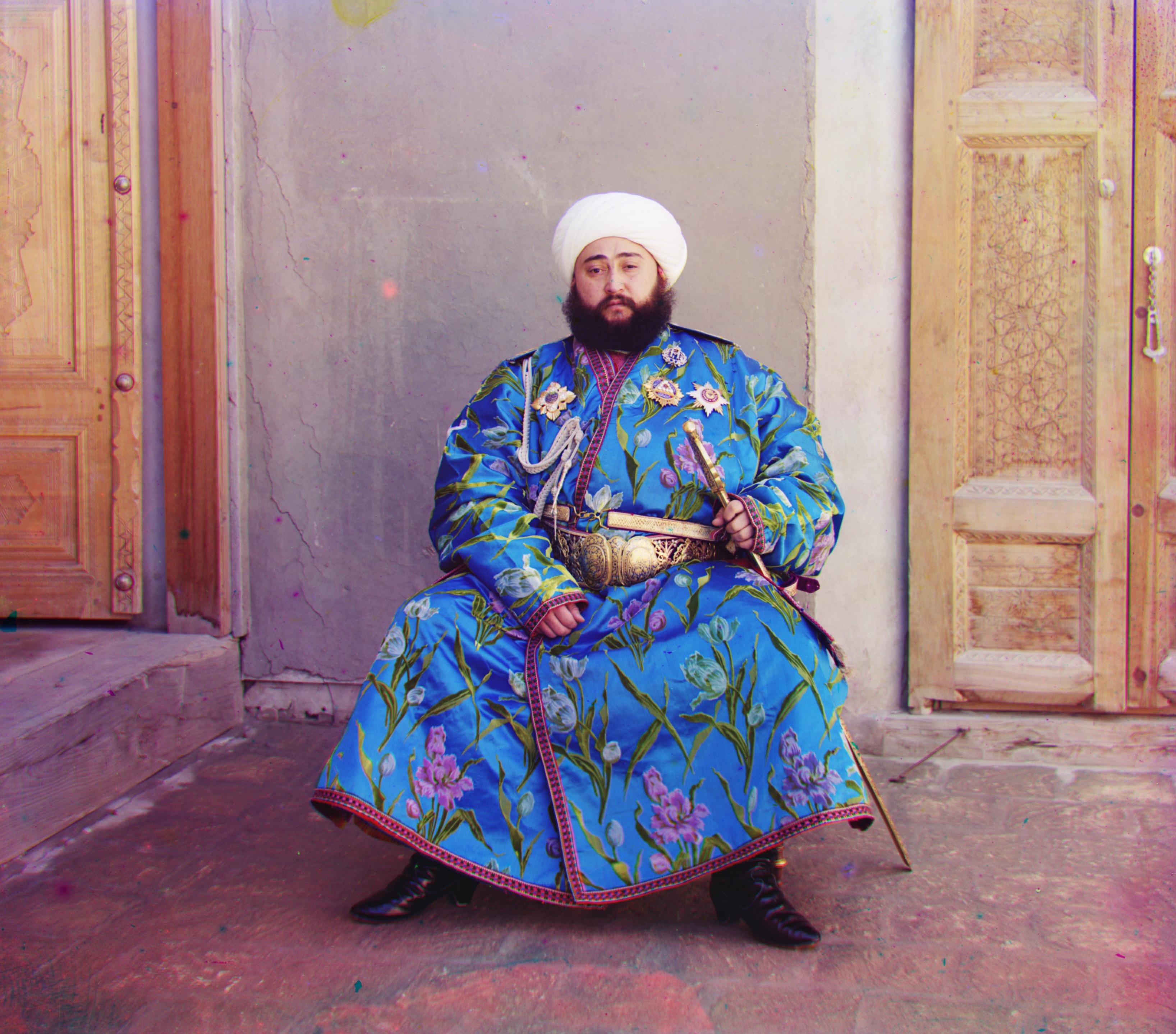
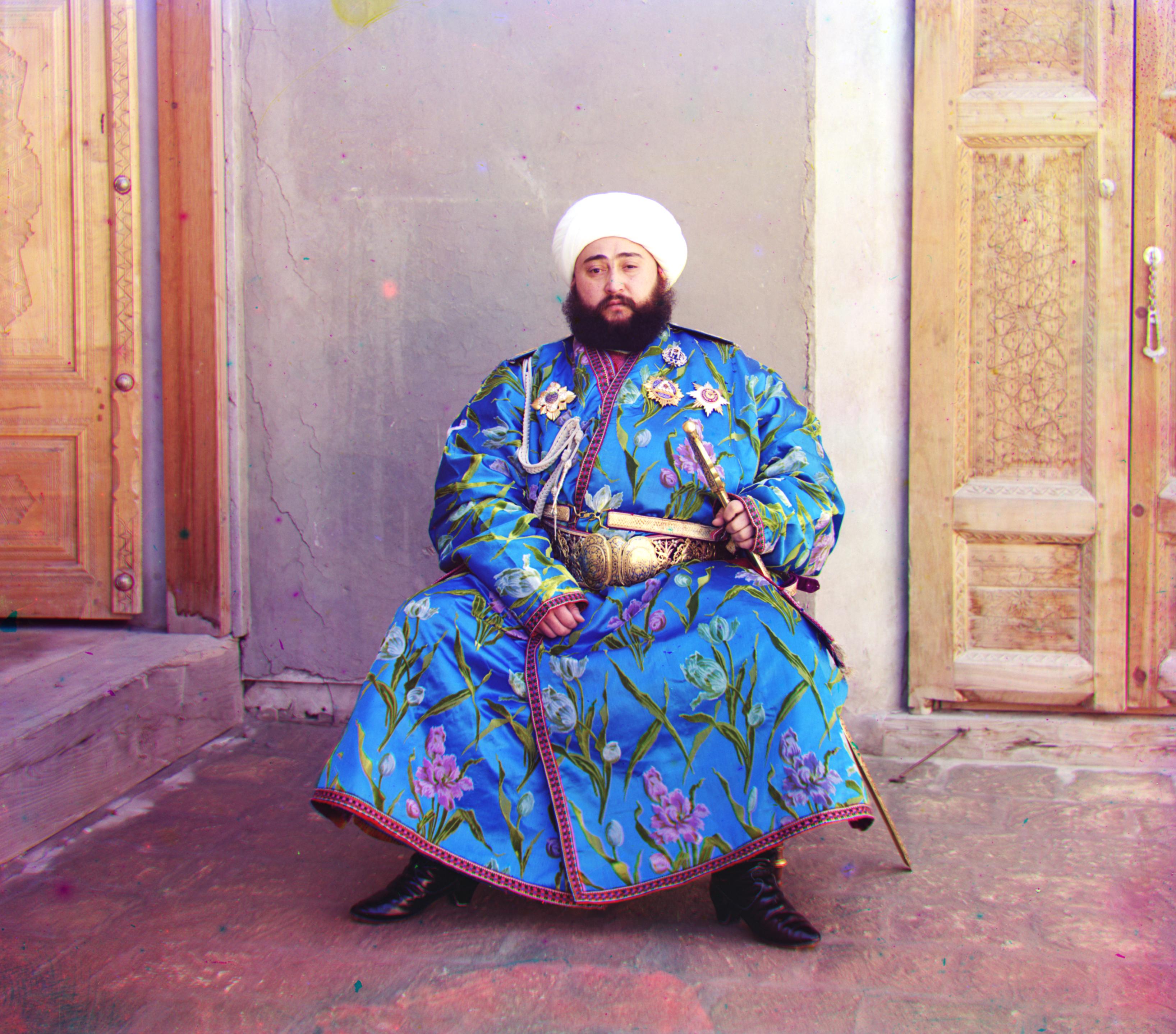
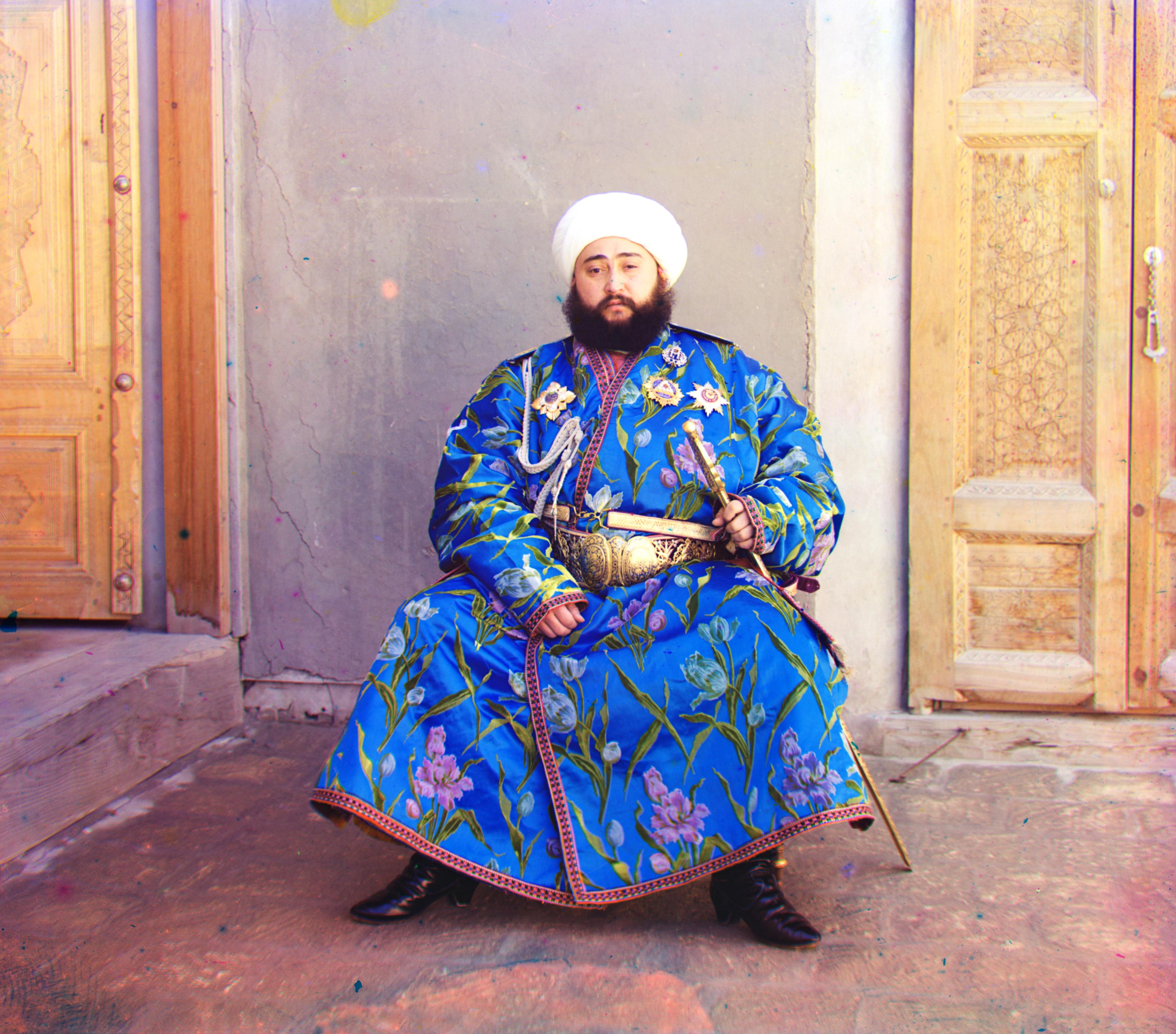
The aforementioned baseline uses NCC over raw pixel space at each pyramid level with exhaustive search, can already achieve reasonable alignment. However, the processed images still contain some artifacts that makes them less visually appealing and not perfectly aligned. For instance, systematic failures can be observed in some TIF images, like the $\texttt{emir.tif}$, where the red channel is obviously mis-aligned (shown below). Therefore, here we analyze and address those systematic failures, and then apply some techniques to enhance the visual quality.
Better Alignment: Robust Metric and/or Feature Space
While the NCC is foundamentally better than SSD due to its normalization, applying it directly on the raw pixel space still makes it highly sensitive to absolute intensities. This results in poor robustness against local defects and outliers (e.g., saturation, scratches, noise), and leads to systematic failures when the channels differ significantly in contrast and brightness.
In $\texttt{emir.tif}$, when we visualize the three channels separately (see below), one can easily observe that the R channel exhibits a highly different contrast and saturation distribution compared to B and G channels. Consequently, NCC on raw intensities tends to systematically mis-align the red channel.
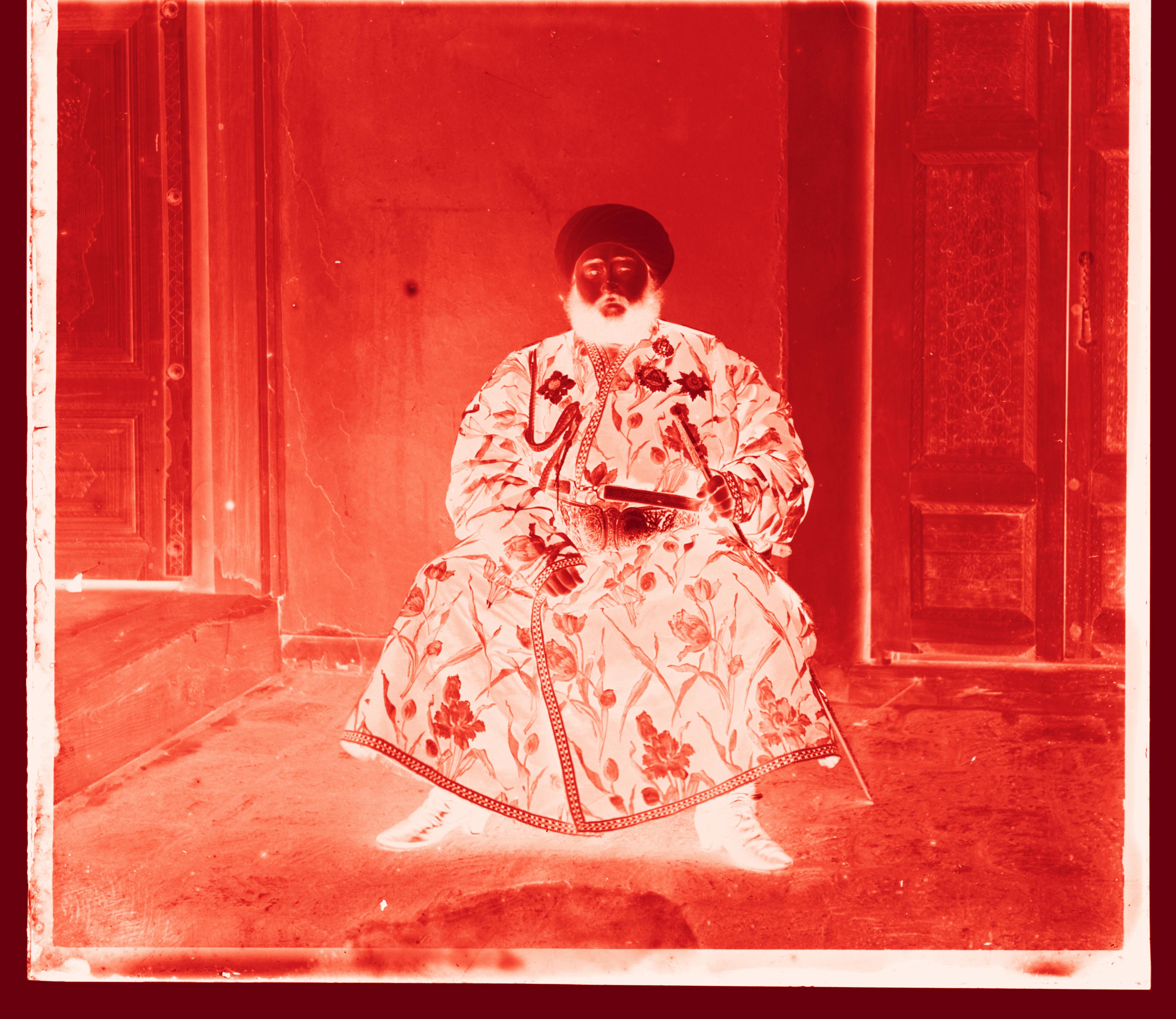
Red channel in red colormap
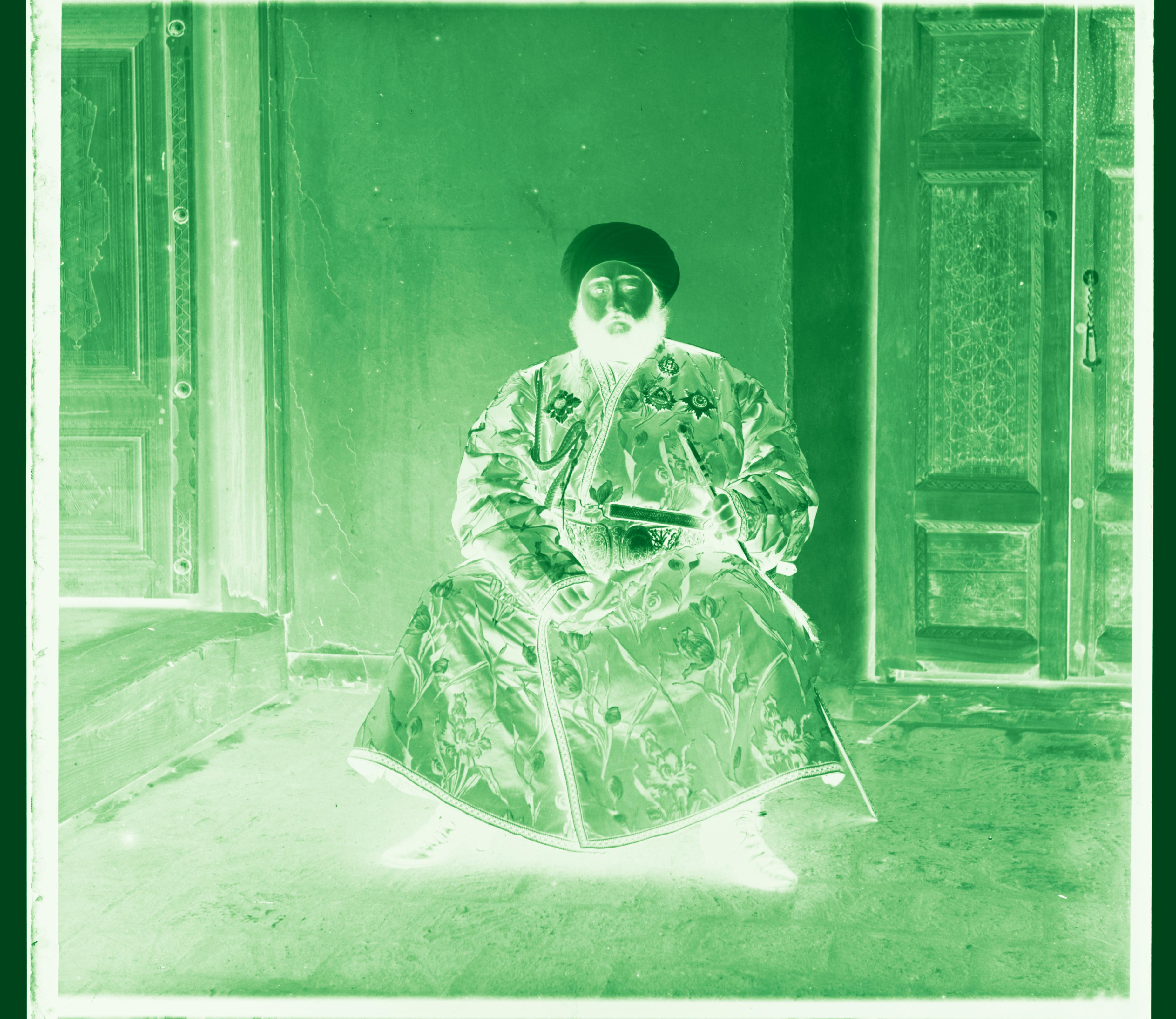
Green channel in green colormap
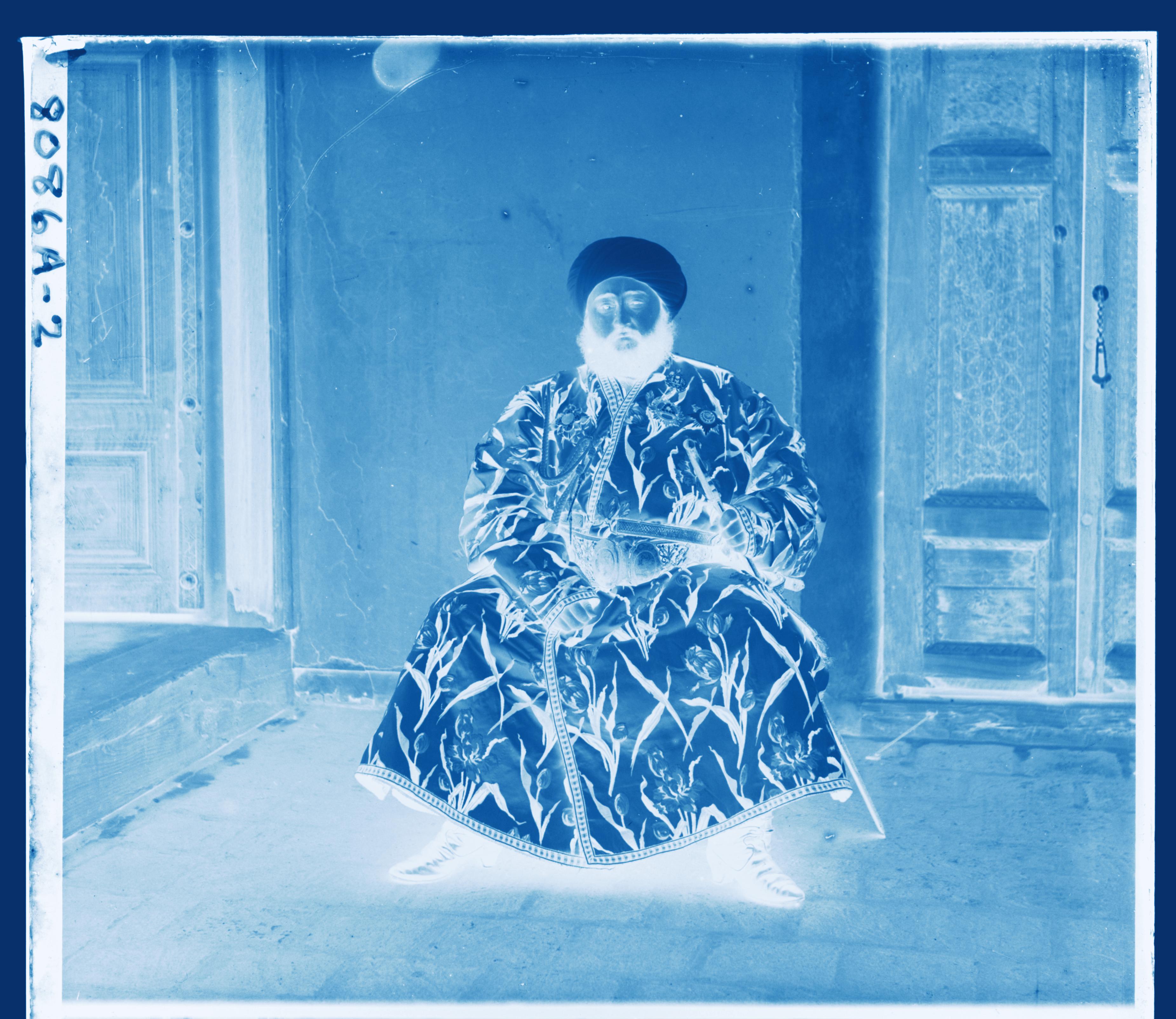
Blue channel in blue colormap
To address this, one can:
- either adopt a more robust metric, or
- map the raw pixel space into feature spaces that are less sensitive to intensity variations.
In my implementation, the latter strategy was adopted. Specifically, I compute NCC in the Sobel gradient space, where the focus is shifted from pixel intensities to edges and structural information. And apparently, the misalignment issue was resolved appropriately.
Results of Multi-Scale Alignment (Exhaustive Search + NCC over Sobel Gradient Space on All Images)
_(2, 5)_(1.50).jpg)
R(3,12) G(2,5) 1.50s
_(4, 25)_(16.50).jpg)
R(-4,58) G(4,25) 16.50s
_(23, 49)_(16.92).jpg)
R(40,107) G(23,49) 16.92s
_(17, 60)_(18.67).jpg)
R(13,123) G(17,60) 18.67s
R(23,90) G(17,42) 17.76s
_(22, 39)_(16.91).jpg)
R(36,77) G(22,39) 16.91s
_(-2, -3)_(18.04).jpg)
R(-8,76) G(-2,-3) 18.04s
_(-17, 41)_(19.10).jpg)
R(-29,91) G(-17,41) 19.10s
_(10, 80)_(17.90).jpg)
R(12,177) G(10,80) 17.90s
_(2, -3)_(1.52).jpg)
R(2,3) G(2,-3) 1.52s
_(29, 78)_(17.53).jpg)
R(37,176) G(29,78) 17.53s
_(-7, 49)_(18.32).jpg)
R(-24,96) G(-7,49) 18.32s
_(12, 54)_(16.96).jpg)
R(8,111) G(12,54) 16.96s
_(2, 3)_(1.52).jpg)
R(3,6) G(2,3) 1.52s
Post-Processing: Automatic Cropping
Once the alignment is done, the colored images often look real enough. However, they typically contain artifacts that reduce their visual quality compared to modern digital photos. Therefore, we here we explore some post-processing techniques to enhance their visual quality.
The most obvious artifact is the borders, which are typically single color and contain (almost) no information. To address this, here we can remove them through automatic cropping.
One method is to analyze the edges of the image. The borders are usually nearly uniform in color, with very few edges along the perpendicular direction. Therefore, with the assumption that "the borders are approximately parallel to the image edges", we can detect them through "finding the location where edge gradient changed dramatically" and crop them out. To improve robustness, we analyze the cumulative distribution of the absolute Sobel gradient values. To achieve this, we can operate on the sobel gradient map with respect to $x$ and $y$ directions separately, details are as follows:
- Convert the image to grayscale to keep only the intensity information
- Compute the Sobel gradient maps with respect to the $x$ and $y$ directions, and take their absolute values
- For each gradient map, project the values by summing along the perpendicular axis (e.g., sum columns for the $x$-gradient)
- Compute the cumulative percentage of these projected values, and crop at the positions where the percentage first exceeds a predefined threshold (e.g., $2\%$)
- To avoid over-cropping the edges where the gradients are not significant (e.g, some clean background), the maximum cropping ratio should be limited by a threshold as well (e.g, $7\%$)
Failure Analysis & Improvement (k-part strategy)
The initial implementation of automatic cropping works well for most images; however, some images contain nose on the borders (e.g., writings that records meta information, rugged edges due to poor preservation), which can be recognized as edges as well. Since the initial cropping method is based on detecting the dramatic change of cumulative edge density, those writings on the border cause the density curve to rise quickly and trigger the threshold too early. However, simply increasing the threshold will cause the cropping to degenerate to "simple crop with a fixed ratio", since most other borders do not contain such writings, and the maximum cropping will be simply controlled by the maximum cropping ratio.
To address this, we can instead adopt a multi-region strategy: instead of applying the cropping detection to the entire image, we divide the image into k vertical (or horizontal) partitions, and perform the same border detection independently on each partition. This is based on the observation that the writings typically appear on a specific region of one border, and the rest of the borders are clean. Therefore, the assumption is that at least one partition will not be heavily influenced by writings or artifacts, and thus can provide a more reasonable cropping boundary. Finally, we take the most aggressive (largest) cropping among the partitions as the final result.
Results of Automatic Cropping (with & without k-part trick)
Some selected results of automatic are demonstrated as follows. One can see that the initial implementation without the k-part trick can already crop the borders appropriately. However, for some cases, the borders cannot beeing cropped cleanly without over-cropping due to noise within borders. For instance, the example one is the case where its right black border contains writings of "5030" at upper part, and the second example shows rugged edges at right and red shades at bottom. After applying aforementioned k-part trick with $k=4$, one can find that the cropped images are cleaner.
Before cropping
.png)
Cropped w/o k-part trick
Cropped w/ k-part trick (k=4)
Before cropping
.png)
Cropped w/o k-part trick
Cropped w/ k-part trick (k=4)
Trade-Off Analysis
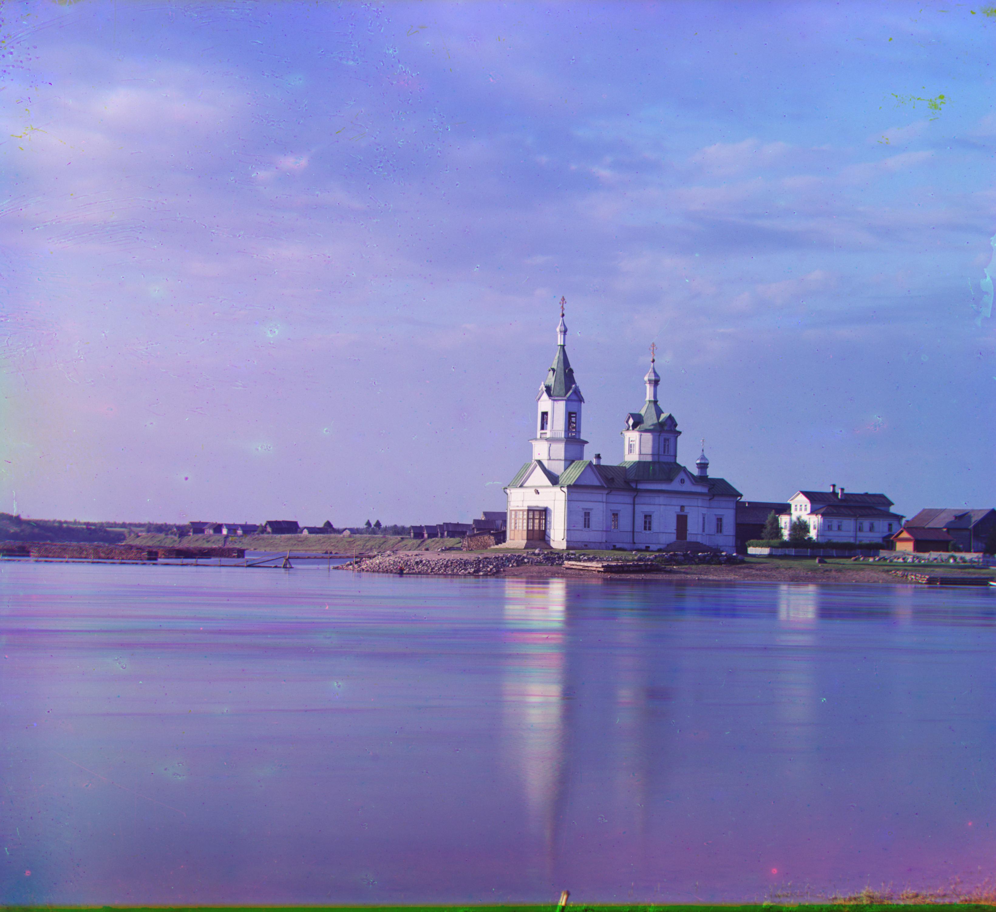
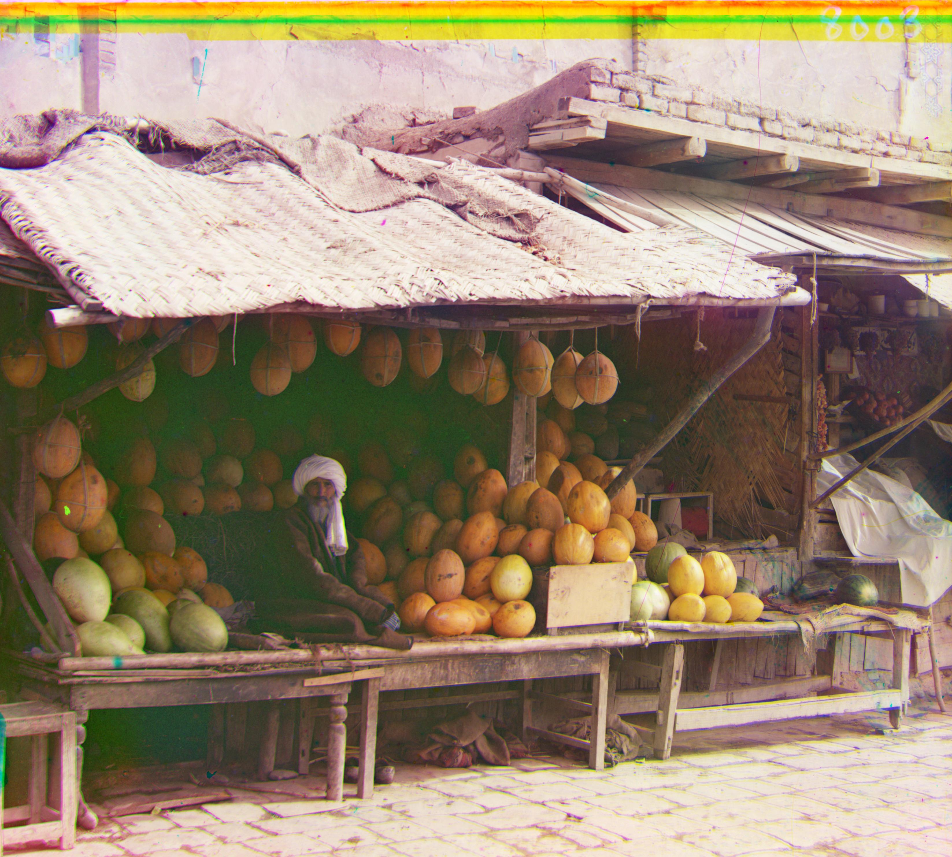
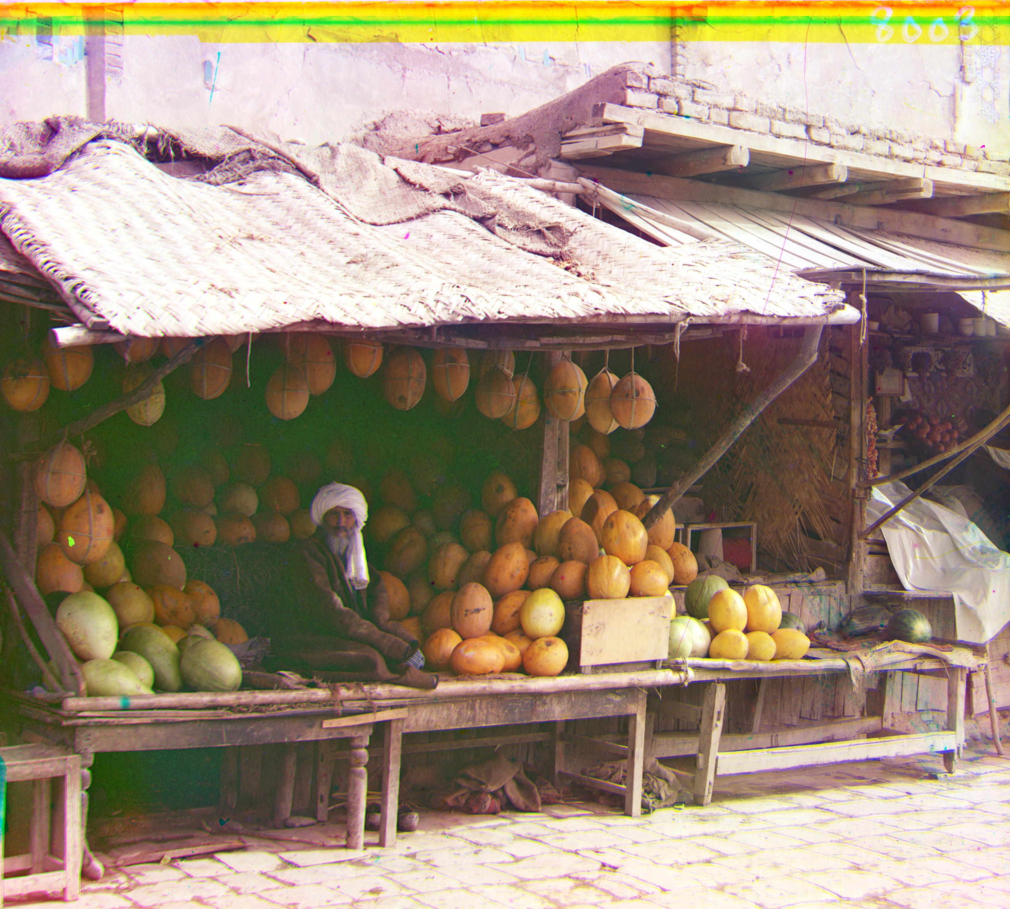
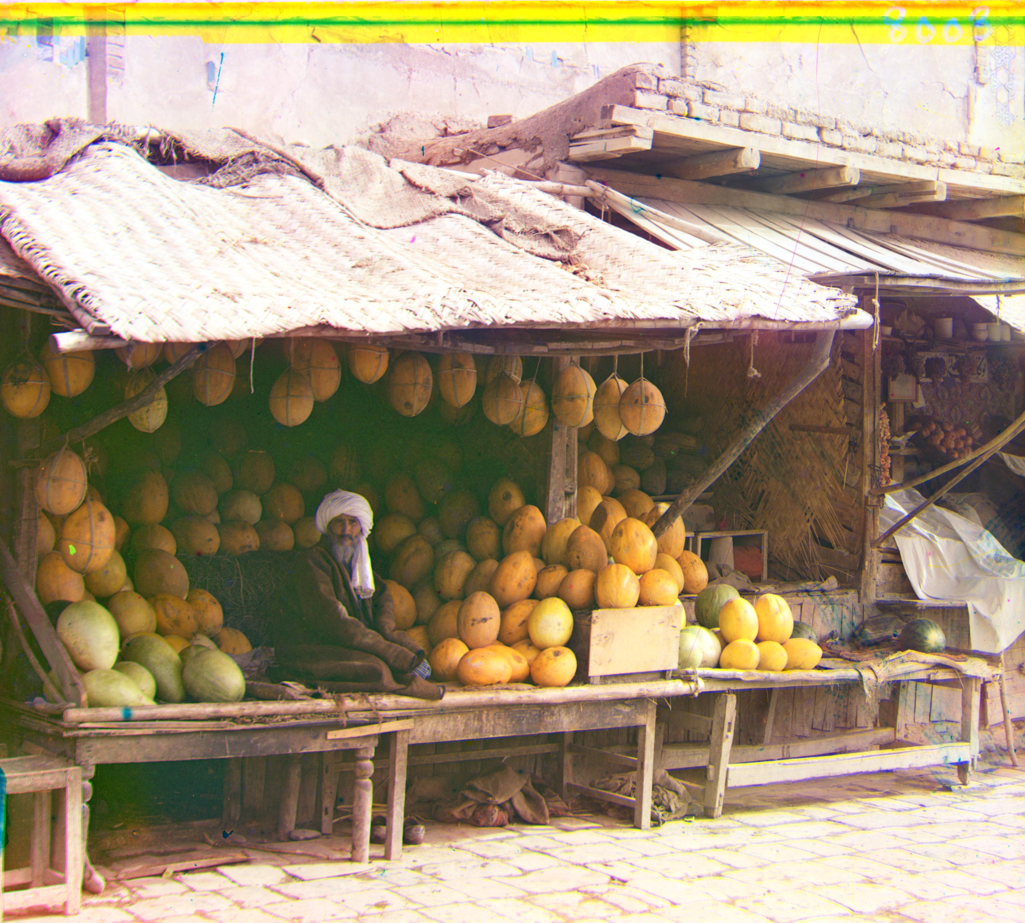
However, there is still a trade-off. After observing the aligned images, one would ask: "How do we define the so-called borders?" Are they just single colored straight bands? Or we should also consider the edge regions that are mainly shaded by single colors while also containing semantic information? Cutting the latter out or adjusting them back to their natural color was a trade-off that took me a long time to consider. The following $\texttt{melons}$ is a good example, it contains a large region of multiple single-colored shaded bands on the top, which apparently is the top of the building behind the fruit farmer; however, if we consider them are borders, they are all cut off and we lose all the information! The ideal way to handle them should be mapping them back to natural colors; however, this seems too hard to automate. Therefore, in my final implementation, I tuned the thresholds to make the cropping not too aggressive, then, we can still keep some of those regions to keep the information inside, even though they may look ugly.
Before cropping
Cropped w/ k-part trick (k=4), keeping some edge regions (top)
Post-Processing: Automatic White Balancing
Limited by the technology of Prokudin-Gorskii's time, the colors of aligned images are typically not natural enough. To enhance the visual quality, here we manipulate the pixel intensities and distributions as post-processing.
From observations, it is common that the aligned colored photos exhibit color casts, i.e., the overall color shifts toward one color. Therefore, to make the colors more natural, here we correct the color through automatic white balancing, where we identify and adjust the white points to be displayed as pure white. Like other color constancy algorithms, white balancing consists of two steps:
- Determining the illuminant under which an image was captured
- Adjusting the colors to counteract the illuminant and simulate a neutral illuminant
There are various algorithms for automatic white balancing, where the most straightforward yet effective ones are the Gray World Assumption and White Patch Assumption. The former assumes that the average reflectance in a scene is achromatic (gray), while the latter assumes that there exists at least one pixel in perfect white (equal RGB values), both of which serves as reference for step 1. Once we have the illuminant information from step 1, correcting the colors (step 2) is simply a linear transformation that scales the RGB channels accordingly.
The linear transformation for adjusting RGB channels can be expressed as a $3 \times 3$ matrix multiplication on the raw RGB values. With the assumption that the image was taken under a single illuminant, and that Prokudin-Gorskii's RGB filters were ideal such that the RGB channels are uncoupled (similar to the Von Kries Coefficient Law that human cones are adjusted separately), then the transformation matrix can be simplified to a diagonal form with per-channel scaling factors:
where $[R', G', B']^{\top}$ are the original RGB values before white balancing, $[R, G, B]^{\top}$ are the adjusted ones. The scaling factors $\alpha, \beta, \gamma$ are determined based on the illuminant estimated from step 1.
But one may ask, which algorithm should we implement for this project? Here we can analyze the photos we have, together with the properties of each algorithm. One common pattern we can observe in Prokudin-Gorskii's collection is that most of them exhibit darkened edges, shadows, or aging artifacts, which bias the global average toward darker or desaturated tones. As a result, applying the Gray World Assumption tends to introduce undesirable color shifts.
On the other hand, by analyzing the subject matter of Prokudin-Gorskii's photographs, we can find that they are mainly landscapes, architecture and humanities, which typically contain some white objects. Therefore, trading off the two algorithms, implementing the White Patch Assumption is a better choice for this project.
Recall that the White Patch Assumption calibrates the photo based on the brightest pixels in each channel, say, $R_{\max}, G_{\max}, B_{\max}$, suppose our intensity range is defined as $[I_{\min}, I_{\max}]$, then the scaling factors can be naively determined as:
However, simply applying the White Patch Assumption on the single brightest pixel of each channel may be sensitive to noise and extreme cases, e.g., some noise pixels are extremely bright, or some images contain saturated regions that are very bright in only one channel, both of which can potentially harm the performance. To address this and enhance the robustness, my implementation involves two strategies:
- Only consider pixels whose channel values are mutually similar (within a threshold $\delta$), which are more likely to be near-white/neutral rather than single-colored highlights.
- Instead of using the single maximum, use the average over the $\texttt{top_p}\%$ brightest pixels (measured in grayscale luminance).
With the constraints above, we now only consider the pixel $i$ that are both bright (i.e., high grayscale intensity $L_i$) and approximately neutral in chromaticity, which are collected into the set:
where $Q_p(L)$ is the threshold corresponding to the $\texttt{top_p}\%$ brightest pixels in the grayscale distribution (set to $\texttt{top_p}=2$ in my implementation, i.e., keep the top $2\%$ brightest pixels), and $\delta$ is the threshold that controls the chromaticity similarity (implemented to be $\delta=0.05$ in my case). Then, the $R_{\max}, G_{\max}, B_{\max}$ are computed as the averages of the corresponding channels over the set $\Omega$:
After scaling, pixels whose intensities exceed the range of $[I_{\min}, I_{\max}]$ are clipped to the nearest boundary.
Results of Automatic White Balancing
Some selected results are shown below. In my implementation, I aimed for a non-aggressive white balancing adjustment, so the $\texttt{top_p}$ and $\delta$ were set to $2$ and $0.05$, respectively. For example, the roof of the fruit farmer and the hat of the Emir were balanced to white appropriately, demonstrating that the method can effectively correct global color casts while preserving a natural appearance.
After Cropping, before WB
After WB
After cropping, before WB
After WB
Post-Processing: Better Color Mapping
There is no need, and indeed it would be incorrect, to assume that Prokudin-Gorskii's RGB filters captured the three channels as accurately as modern cameras do. Therefore, we require a mapping to correct the systematic color cast caused by these filters. This means that the diagonal matrix used in white balancing is not sufficient; there should also be coupling effects between channels. Here, I implement a simple linear color mapping, following the same approach as in white balancing, namely a $3 \times 3$ matrix multiplication on the raw RGB values. However, instead of being diagonal, the transformation matrix is now full. This color remapping is applied after white balance in my pipeline; thus, assuming that the white-balanced images are already neutral, the mapping should not affect neutral colors (gray or white). The transformation matrix is therefore defined as:
which ensures that each row sums to 1, so any input neutral color ${R=G=B}$ remains neutral after transformation. Since we don't have a "ground truth" for optimizing the parameters, here I tune the parameters manually based on reference photographs and visual inspection (e.g., correcting white walls, blue skies, and earthy tones). Although somewhat subjective, this method consistently improves the perceptual realism of the reconstructed images.
Results of Automatic White Balancing
Some selected results are shown below. My final implemented parameters are: $a=-0.12$, $b=-0.15$, $c=0.30$, $d=-0.08$, $e=0.02$, $f=0.00$.
After cropping + WB, before color remapping
After color remapping
After cropping + WB, before color remapping
After color remapping
Post-Processing: Automatic Contrasting
Another common issue in Prokudin-Gorskii's collection is low-contrast, which means, the image histograms are not spanning the full intensity range, yielding details in some regions less distinguishable. Therefore, subsequent contrast adjustment is necessary to make weak signals more visible, revealing details that were already present in the data but previously hidden in low-contrast regions. Here we enhance the contrast by manipulating the image histograms.
The simplest way is to map the histogram linearly to span the full intensity range, namely contrast stretching. Say, for the grayscale space with the intensity range of $[I_{\min}, I_{\max}]$ and total number of gray levels $LI$ (e.g., for uint8, $LI=256$ and range is $[0,255]$), if we want to stretch an image, whose maximum and minimum intensities are $r_{\max}$ and $r_{\min}$, then the function mapping the original intensity $r$ to the new one $s$ (assuming $I_{\min}=0$ and $I_{\max}=LI-1$) is defined as:
However, one can observe that this method is sensitive to noise and outliers, since it relies on $r_{\min}$ and $r_{\max}$ heavily, hence, any noise/outliers that deviate off the main distribution will affect the result significantly. Moreover, such a linear mapping does not change the shape of histogram, therefore, cannot effectively enhance regions where pixel intensities are densely clustered (i.e., locally low-contrast regions due to over/under exposure).
A more robust way is histogram equalization (HE), which manipulates the cumulative distribution function (CDF) of the pixel intensities. Starting from the image histogram, one can normalize it to get the probability distribution function (PDF) and then get the CDF through cumulative summation, which is basically the empirical CDF (ECDF) of the pixel intensities, defined as:
where $R_i$ is the intensity of pixel $i \in \{1,2,...,n\}$ that belongs to one of $n$ pixels of the image, and $\mathbf{1}(\cdot)$ is the indicator function.
Then, we can use ECDF to construct the mapping function from original intensity $r$ to new intensity $s$ that satisfies the requirement that $T: [I_{\min}, I_{\max}] \to [I_{\min}, I_{\max}]$, which is simply a scaled version of ECDF:
From the definition, one can observe that this method is less sensitive to outliers, and can redistribute the pixel intensities more evenly, hence, able to address the aforementioned issues of contrast stretching.
However, it still has limitations in our case:
- Both of above methods operate globally, however, the photos we have typically contain noise and defects in some local regions (e.g., uneven aging artifacts and unusual monochrome shades around the edges). Such local defects and noise will be incorporated into the new histogram, propagated to the whole image, and affect the overall contrast enhancement.
- Since HE redistributes pixel intensities to approximate a uniform distribution, originally dense regions may be excessively spread out, while sparse regions are filled with additional pixels, sometimes introducing artificial contrast patterns or visual artifacts.
With such issues in mind, the final implementation adopts the Contrast Limited Adaptive Histogram Equalization (CLAHE), which:
- Operates HE on small tile regions locally and combines the results via bilinear interpolation, addressing the first issue.
- To alleviate the second issue, HE on each tile is operated on a clipped and re-distributed histogram (through a parameter $\texttt{clip_limit}$), yielding better local contrast enhancement without over-amplifying noise.
Luckily, skimage provides a well-implemented function for CLAHE, so I used $\texttt{skimage.exposure.equalize_adapthist}$ for my final implementation.
Results of Automatic Contrasting
Some selected results are shown below. Again, to avoid over-enhancement, I set the parameter $\texttt{clip_limit}$ to be a small value ($0.004$). One can see that after applying CLAHE, the details in some low-contrast regions are revealed, e.g., the texture of the fruit, and the details of Emir's beautiful cloth.
After cropping + WB + remapping, before contrast
After CLAHE
After cropping + WB + remapping, before contrast
After CLAHE
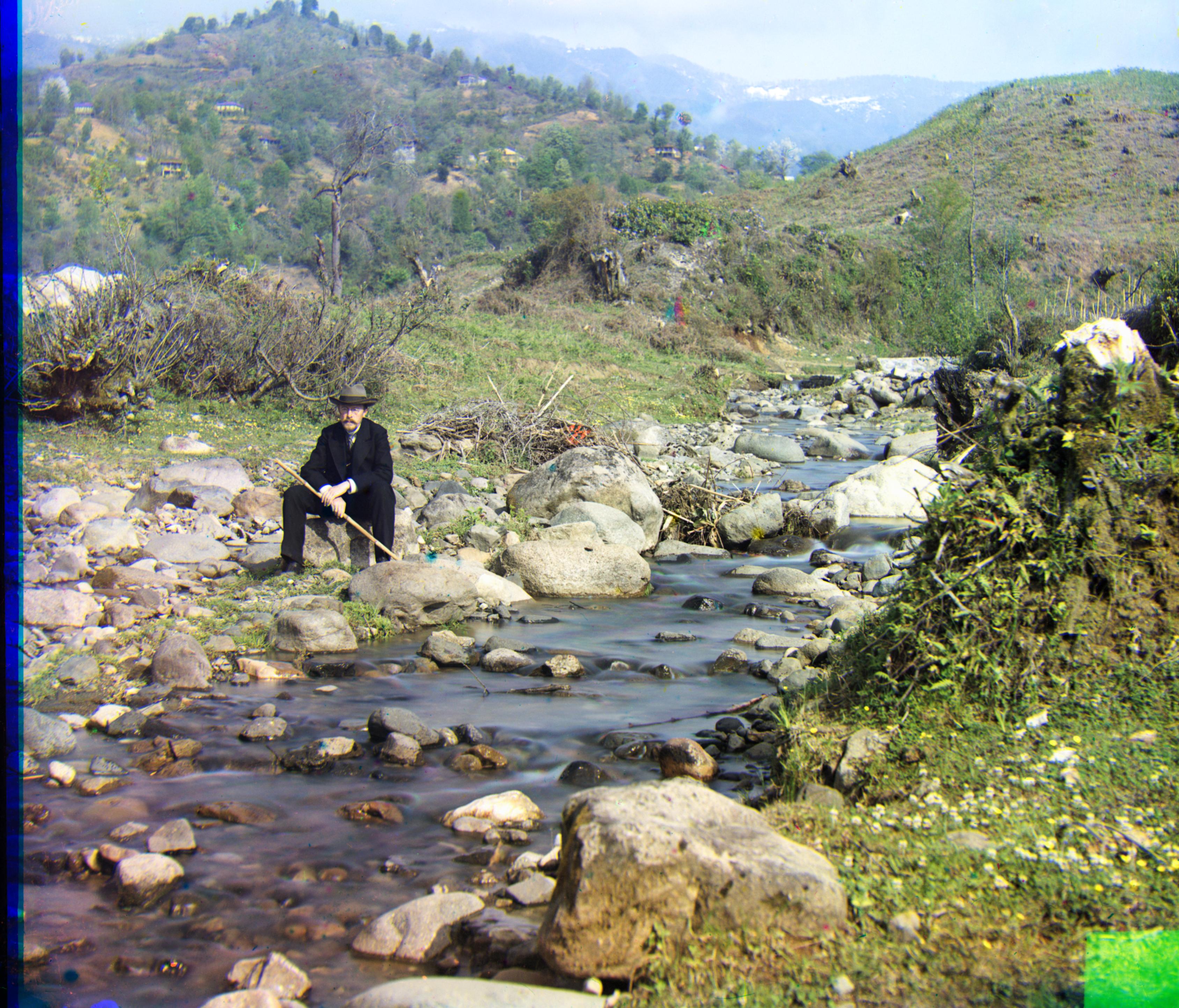
Results of Final Pipeline (Alignment + Pyramid + Sobel $\to$ Cropping $\to$ WB $\to$ Color Remapping $\to$ Contrast)
Finally, let's implement aforementioned algorithms and pre-/post-processing techniques to process the 14 images at hand, which are shown below. The run time only considers the alignment step, excluding post-processing.
R(3,12) G(2,5) 1.50s
R(-4,58) G(4,25) 16.50s
R(40,107) G(23,49) 16.92s
R(13,123) G(17,60) 18.67s
R(23,90) G(17,42) 17.76s
R(36,77) G(22,39) 16.91s
R(-8,76) G(-2,-3) 18.04s
R(-29,91) G(-17,41) 19.10s
R(12,177) G(10,80) 17.90s
R(2,3) G(2,-3) 1.52s
R(37,176) G(29,78) 17.53s
R(-24,96) G(-7,49) 18.32s
R(8,111) G(12,54) 16.96s
R(3,6) G(2,3) 1.52s
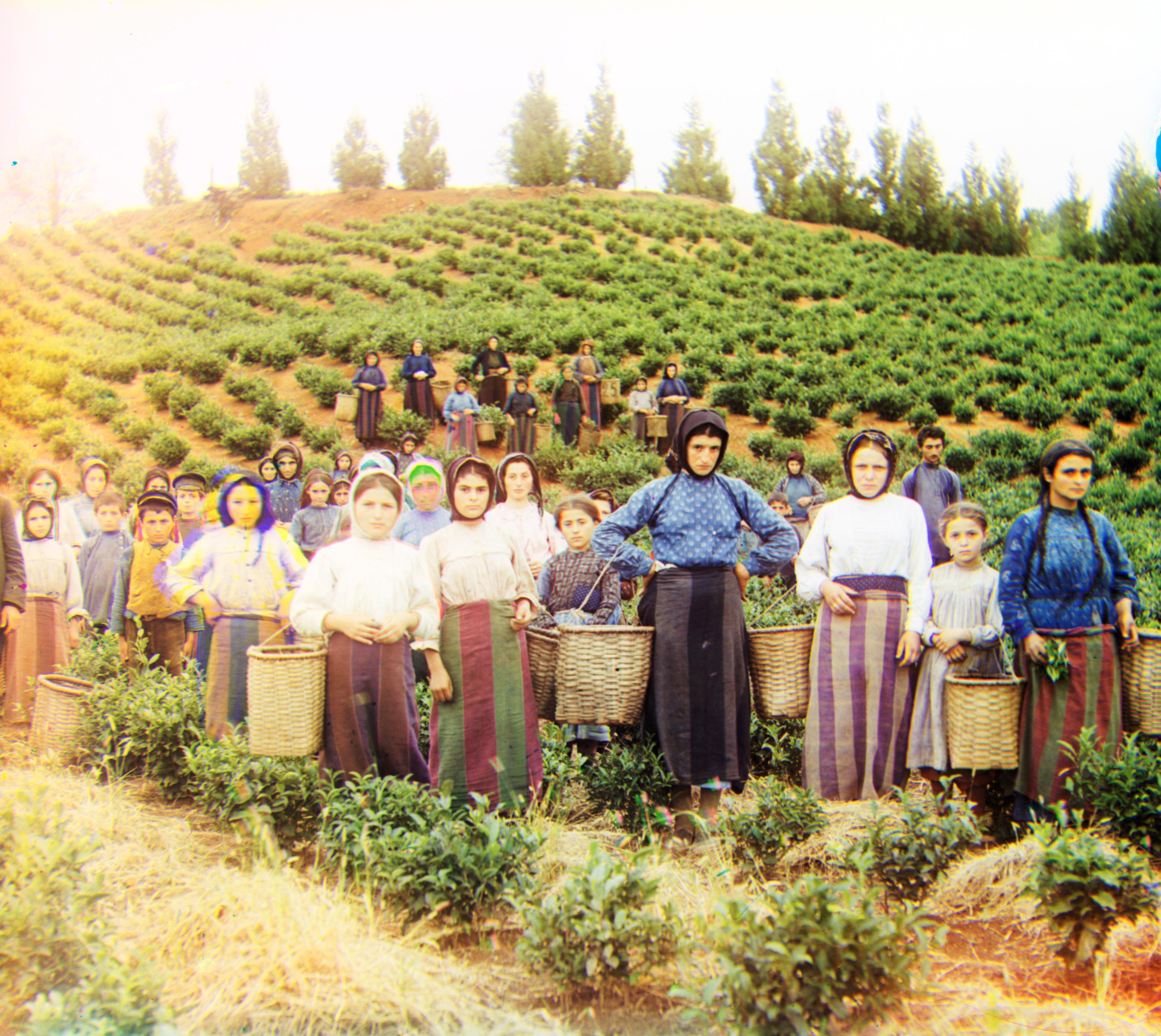
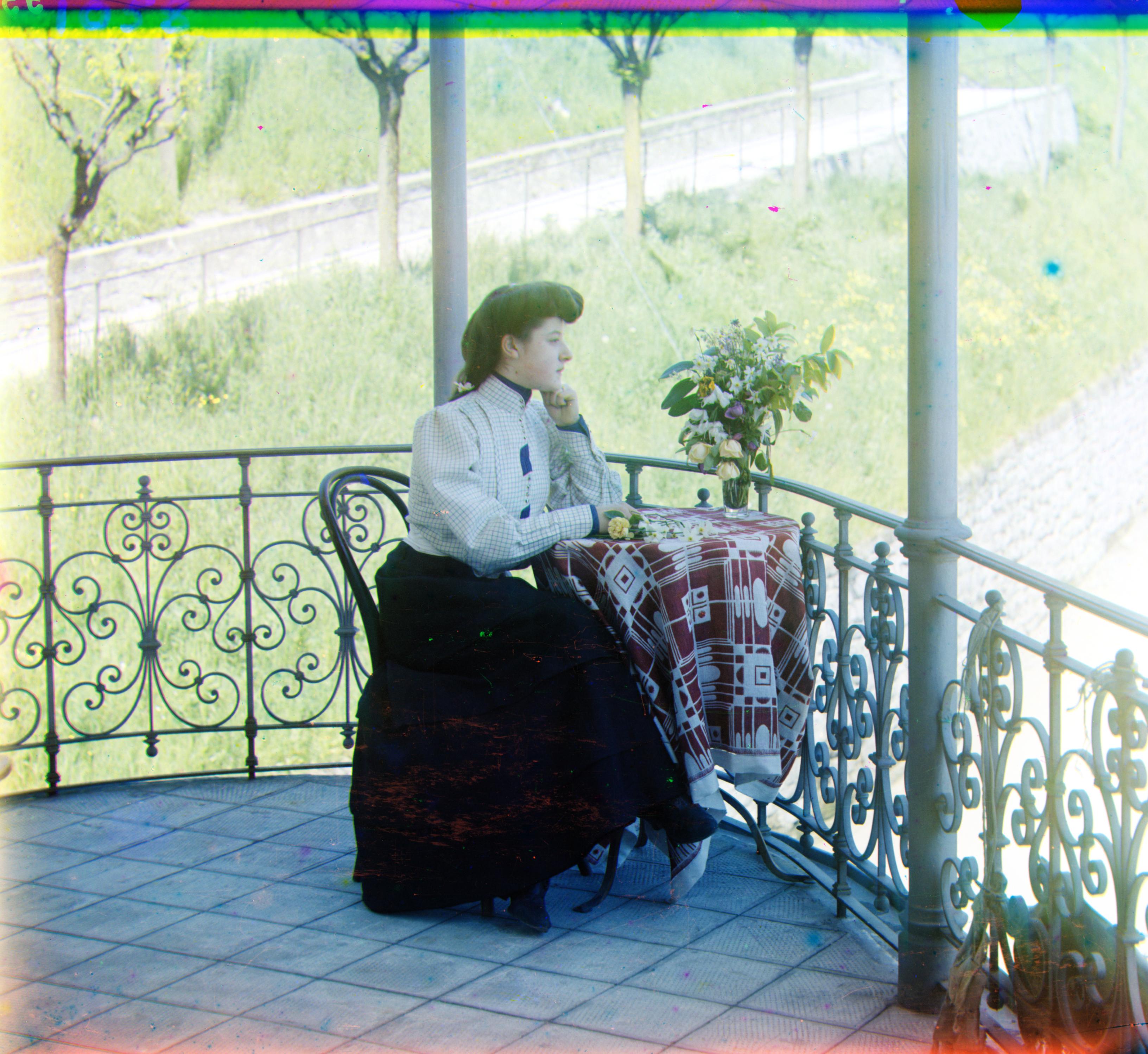
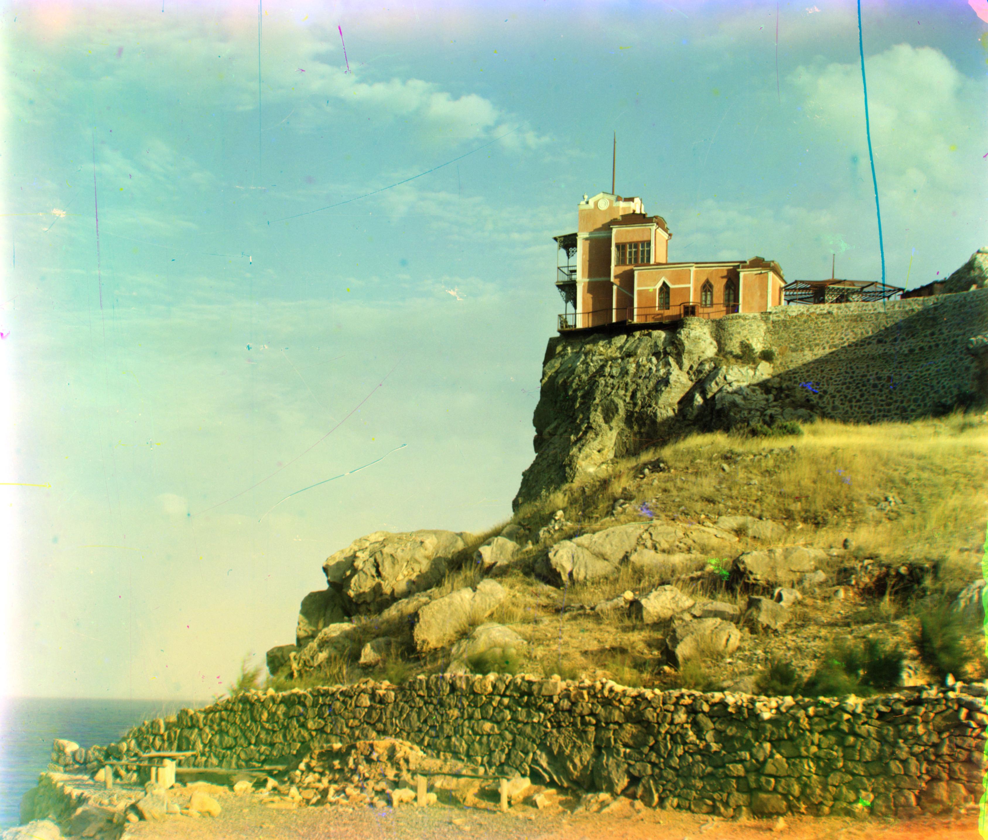
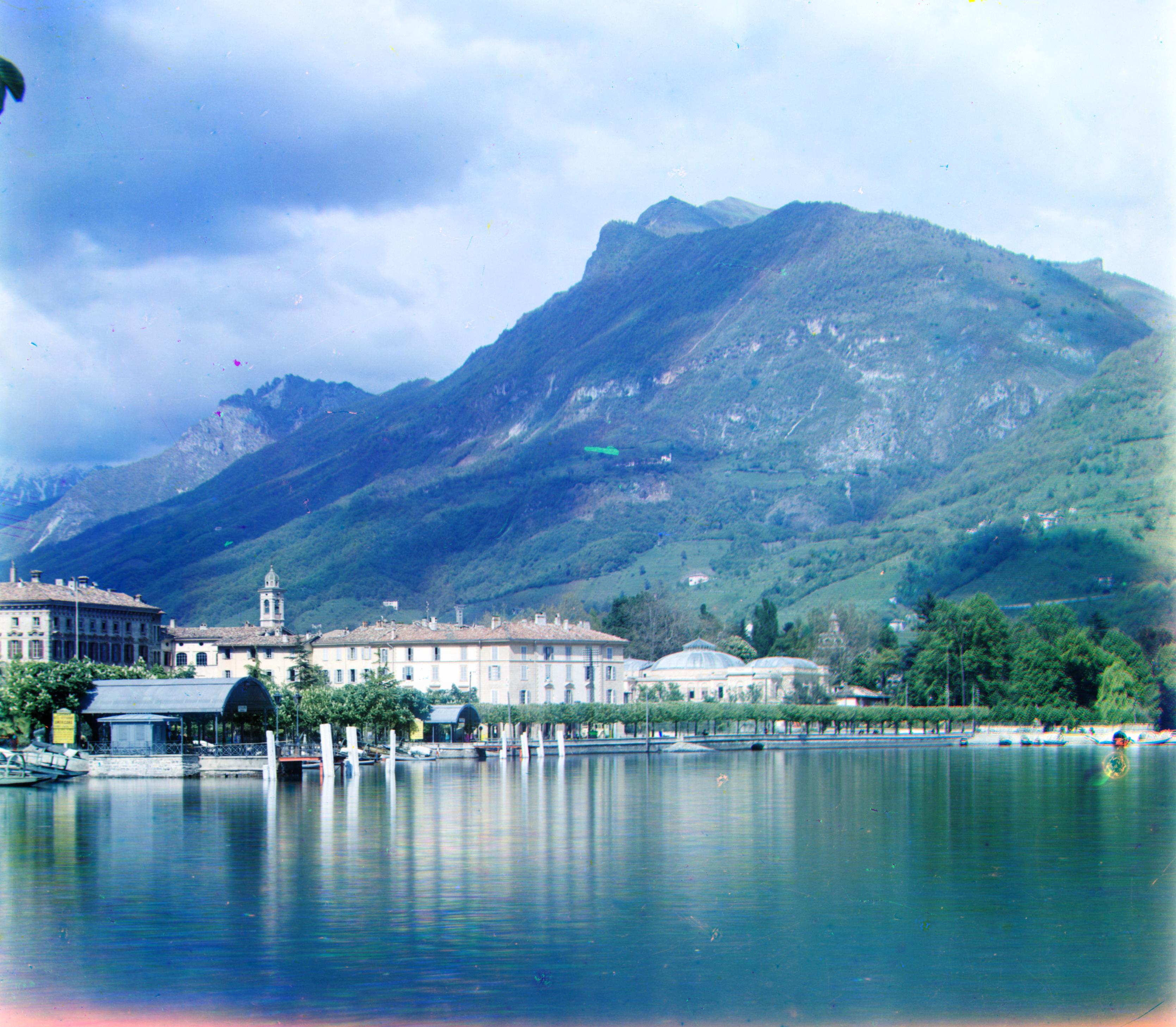
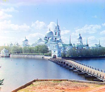
Performance on My Own Selections (looks good :D)
As a structural engineer, I selected some photos of structures (buildings and bridges) to test the performance and robustness of my algorithm, and they all look good to me!