Fun With Diffusion Models!
Introduction
In this project, we explore diffusion models for generative image tasks. Part A focuses on understanding and experimenting with diffusion sampling, including forward and reverse processes, classical and learned denoising, classifier-free guidance, image-to-image translation, inpainting, and multi-view optical illusions. These techniques allow us to understand how modern diffusion models generate and edit images. Then, in part B, we will build and train our own flow matching model on MNIST.
Highlights
- Diffusion models for image generation
- Forward & Reverse Sampling Loops
- Classical, One-Step, and Iterative Denoising
- Classifier-Free Guidance
- Image-to-image Translation (SDEdit)
- Inpainting and Shape Completion
- Visual Illusions & Hybrid Images
- Flow Matching Models
Part A: The Power of Diffusion Models!
In part A, we will play with pretrained diffusion models to perform various image generation tasks and sampling techniques. We will use the DeepFloyd IF diffusion model here. All implementations will follow the instructions in the provided notebook and project page.
A.0: Setup & Play with DeepFloyd
Once we have access to DeepFloyd through Hugging Face, we can start playing with this model by sampling images conditioned on our self-crafted text prompts. The text prompts were encoded via a pretrained text encoder, in this case, the encoder of a T5 model was used, which embeds each plain text prompt into a $[1, 77, 4096]^{\top}$ vector, where $77$ is the maximum token length (sentences longer than this will be truncated) and $4096$ is the embedding dimension. The text embeddings are then fed into the diffusion model to guide the image generation process.
Experiment: Effect of num_inference_steps
Let's generate some images using DeepFloyd conditioned on some of
our text prompts. Recall that the
num_inference_steps will affect the quality and
diversity of generated images, so here we will explore different
values to observe their impact.
All Part A experiments were generated using seed=100 (as shown in figures).
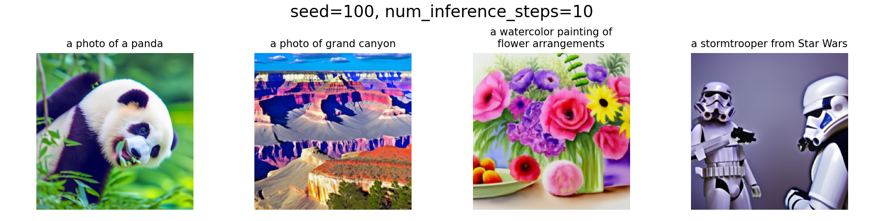
From the results above, we can see that with a low number of
num_inference_steps, e.g., 10, the generated image will
be of low quality and may not fully ground on the text prompt. For
instance, the The panda's body is in an unnatural posture, and we
got $2$ stormtroopers instead of $1$ as specified in the prompt. As
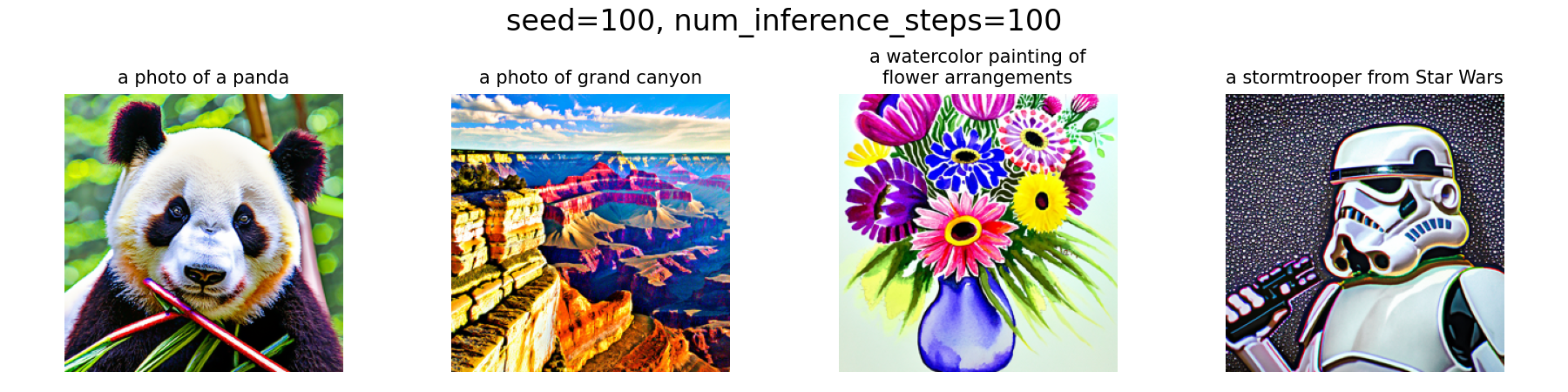
we increase the number of inference steps, say, to $100$, the image
quality improves significantly and the details align better with the
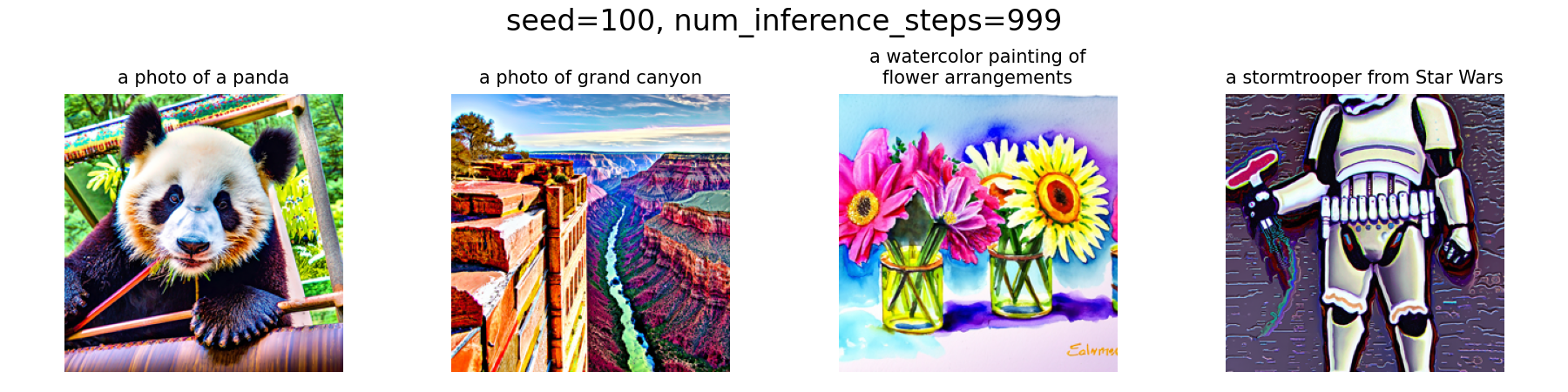
prompt. However, this improvement in quality will have certain
marginal benefits, which can be proved by the fact that further
increasing the steps to $999$ does not yield a substantial
improvement compared to $100$ steps.
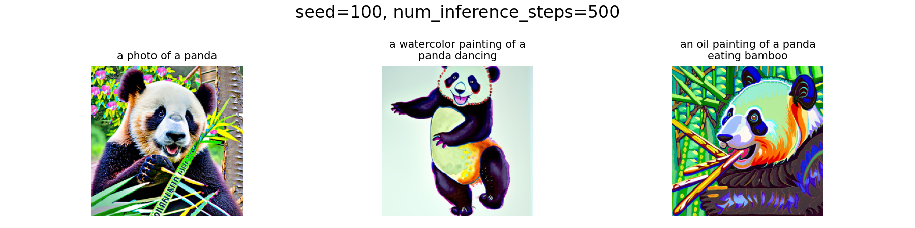
Experiment: Effect of Prompts
Beyound num_inference_steps, text prompts for the same
sense of image with varying details will also affect the generated
results, so let's try a few different prompts for our panda. One can
observe that once the num_inference_steps is set to a
reasonably large value (e.g., $500$), the generated images will be
well aligned with the prompts, demonstrating the model's strong
capability in grounding textual descriptions to visual content.
A.1: Sampling Loops
In this part, we will implement our own "sampling loops" that use the pretrained DeepFloyd denoisers, which should produce high-quality images such as the ones generated before. We will then modify these sampling loops to solve different tasks, such as inpainting or producing optical illusions.
Starting with a clean image $x_0$, we can iteratively add noise to an image, obtaining progressively noisier images $x_1, x_2, \ldots, x_t$, until we are left with pure noise at timestep $t=T$, hence, $x_0$ is our clean image, and for larger $t$ more noise is in the image.
A diffusion model reverses this process by denoising the image through predicting the noise component given a noisy $x_t$ and the timestep $t$. Each iteration, we can either remove all noise in one step, or remove a small amount of noise, obtaining a slightly cleaner image $x_{t-1}$, and repeat this process until we reach $x_0$. This means we can also start from pure noise $x_T$ and iteratively denoise it to obtain a clean image $x_0$.
For the DeepFloyd models, $T=1000$, and the exact amount of noise added at each step is dictated by noise coefficients $\bar{\alpha}_t$, which were chosen by the people who trained the model.
A.1.1: Forward Process
As the key part of diffusion, here we first implement the forward process, i.e., take a clean image and add noise to it, defined by: $$ q(x_t \mid x_0)=\mathcal{N}\left(x_t ; \sqrt{\bar{\alpha}_t} x_0, (1-\bar{\alpha}_t) \mathbf{I}\right),\tag{A.1}$$ which is equivalent to computing $$ x_t = \sqrt{\bar{\alpha}_t} x_0 + \sqrt{1 - \bar{\alpha}_t} \epsilon, \quad \epsilon \sim \mathcal{N}(0, 1).\tag{A.2}$$ Therefore, for a given clean image $x_0$ and timestep $t$, the noisy image $x_t$ can be obtained by sampling $\epsilon$ from a standard normal distribution and adding it to the scaled clean image.
Implementation & Results
The
Campanile
at noise levels of [250, 500, 750] through a
forward function (implemented following the
aforementioned equations) are visualized below. As expected, the
images become increasingly noisy as the timestep increases.
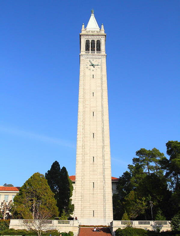
![Campanile at t=[0,250,500,750]](media/part-a/a1-1_seed100_levels.png)
t = [0,250,500,750] (seed = 100)
A.1.2: Classical Denoising
Before denoising with the learned diffusion model, let's first see
how classical methods perform. Here, we use
Gaussian blur filtering to try to remove the noise in the
noisy images that we obtained before. The results images before and
after denoising are shown below. In my implementation, I used
sigma = 2 and
kernel_size = 6 * sigma + 1 for the Gaussian filter,
i.e., covering over $99$% mass of the Gaussian density. Apparently,
the Gaussian blur is ineffective at removing this level of noise.
This can be mainly attributed to the fact that those noisy images
have lost high-frequency structure, while blurring only smooths the
image, hence, it cannot reconstruct lost details.
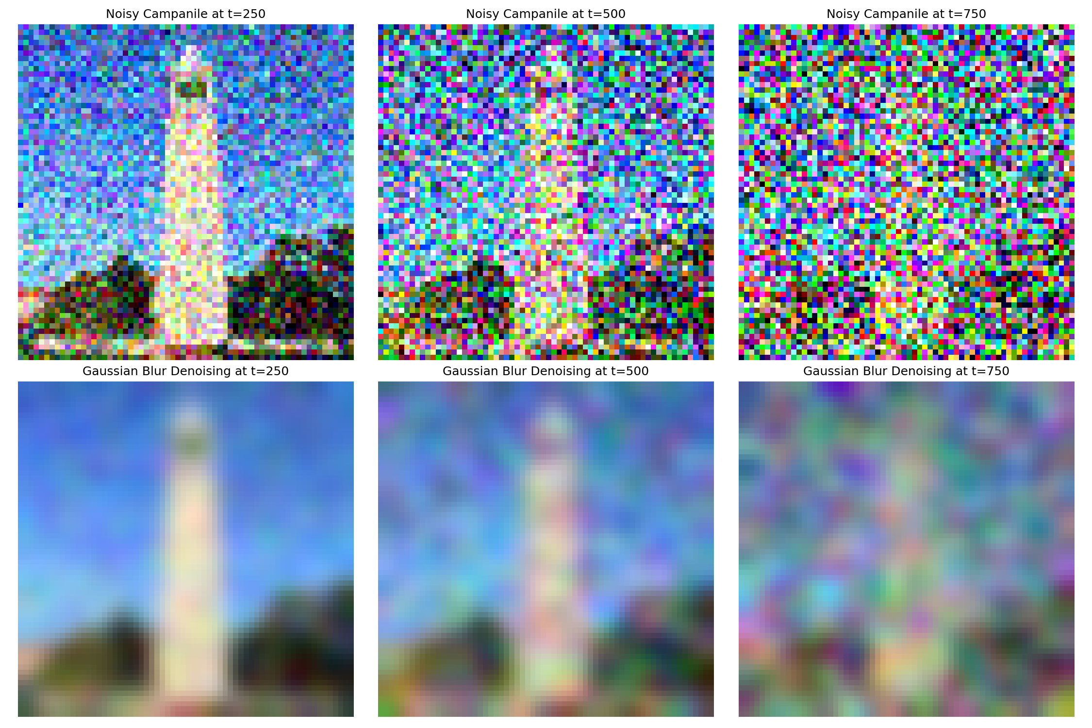
t = [250,500,750] (seed = 100)
A.1.3: One-Step Denoising
Now, let's use the pretrained diffusion model to perform the same denoising task in one step. Since the model is pretrained on a very large dataset of $(x_0, x_t)$, we can use it to recover the Gaussian noise conditioned on a certain timestep $t$ and remove it.
For matching the input format of the model, since it was trained with text conditioning, we provide the embedding of the prompt "a high quality photo" as a neutral conditioning.
Implementation & Results
Again, the same noisy images at timesteps
t = [250, 500, 750] are denoised using the one-step
denoising function we implemented. The results are shown below,
which demonstrate a significant improvement over classical Gaussian
denoising. The pretrained diffusion model effectively recovers much
of the lost detail and structure in the images. However, with the
increase of noise level, some artifacts start to appear in this
one-step approach, indicating that a single denoising step may not
be sufficient for very noisy cases.
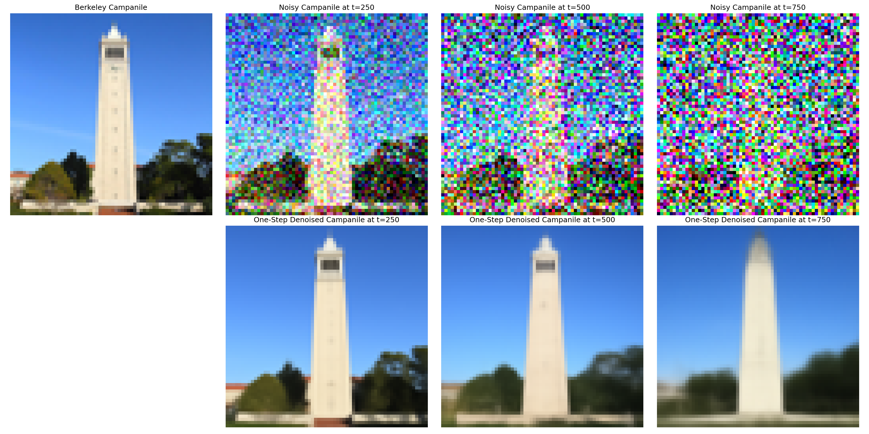
One-Step Denoising Results on Campanile at
t = [250,500,750] (seed = 100)
A.1.4: Iterative Denoising
In part A.1.3, we saw that one-step denoising by the diffusion model does a much better job than classical approaches such as Gaussian blur. However, we also noticed that it does get worse as we add more noise, which makes sense, as the problem is much harder with more noise!
To address this, recall that diffusion models are designed to denoise iteratively, so here we implement an iterative denoising loop that gradually removes noise over multiple steps.
In theory, we could start with $x_{1000}$ at timestep $T=1000$, denoise one step each iteration, and carry on until we reach $x_0$. However, such a long chain will hinder efficiency, so instead, we can actually speed things up by skipping steps, whose theoretical foundation can be found in this article.
To skip steps, we can define a new list of timesteps called
strided_timesteps, which is a subset of the original
timesteps, hence, strided_timesteps[0] corresponds to
the largest $t$ (and thus the noisiest image), and
strided_timesteps[-1] corresponds to $t=0$ (the clean
image). In my implementation, the stride was set to $30$.
On the i-th step, i.e.,
$t=$strided_timesteps[i], we denoise the image to
obtain a less noisy image $t'=$strided_timesteps[i+1],
the calculation follows: $$ x_{t'} =
\frac{\sqrt{\bar\alpha_{t'}}\beta_t}{1 - \bar\alpha_t} x_0 +
\frac{\sqrt{\alpha_t}(1 - \bar\alpha_{t'})}{1 - \bar\alpha_t} x_t +
v_\sigma,\tag{A.3} $$ where:
- $x_t$ is our image at timestep $t$
- $x_{t'}$ is our noisy image at timestep $t'$ where $t' < t$ (less noisy)
- $\bar\alpha_t$ is defined by
alphas_cumprod - $\alpha_t = \bar\alpha_t / \bar\alpha_{t'}$
- $\beta_t = 1 - \alpha_t$
- $x_0$ is our current estimate of the clean image (computed using the one-step denoising formula from the previous section).
The $v_{\sigma}$ is the additional noise term predicted by
DeepFloyd, added via the provided
add_variance function.
Implementation & Results
Here we first create the strided_timesteps by the
following snippet:
Code Snippet:
create strided_timesteps
strided_timesteps = list(range(990, -1, -30))
Then, starting with the given function framework in the notebook, we
can implement the iterative denoising loop, which simply follows the
equation derived above. With i_start = 10, the noisy
Campanile every $5$th loop of denoising is shown below, where we can
see that they becomes gradually cleaner.
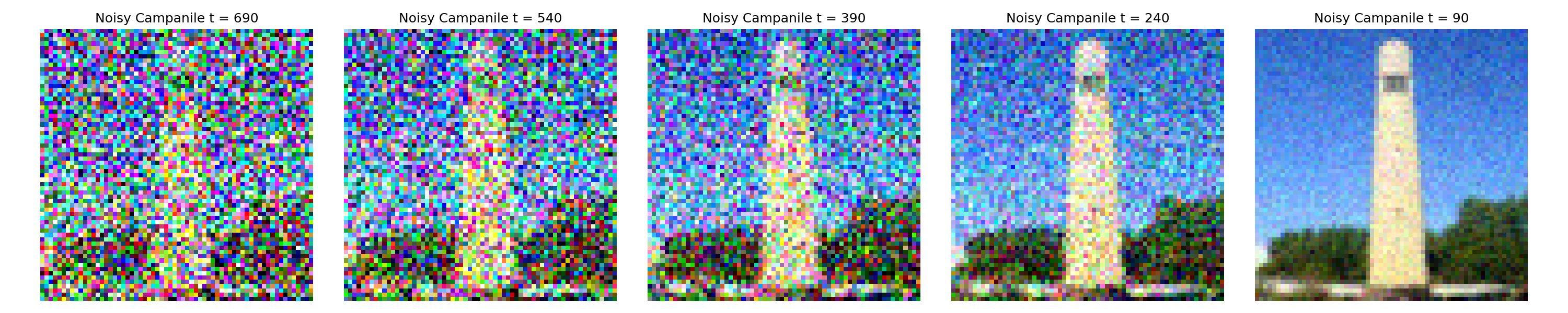
i_start = 10 (seed = 100)
As a comparison, the original image and final denoised images after the aforementioned approaches are shown below, and we can see that the iterative denoising produces the best results, effectively recovering fine details and structure from the noisy input.
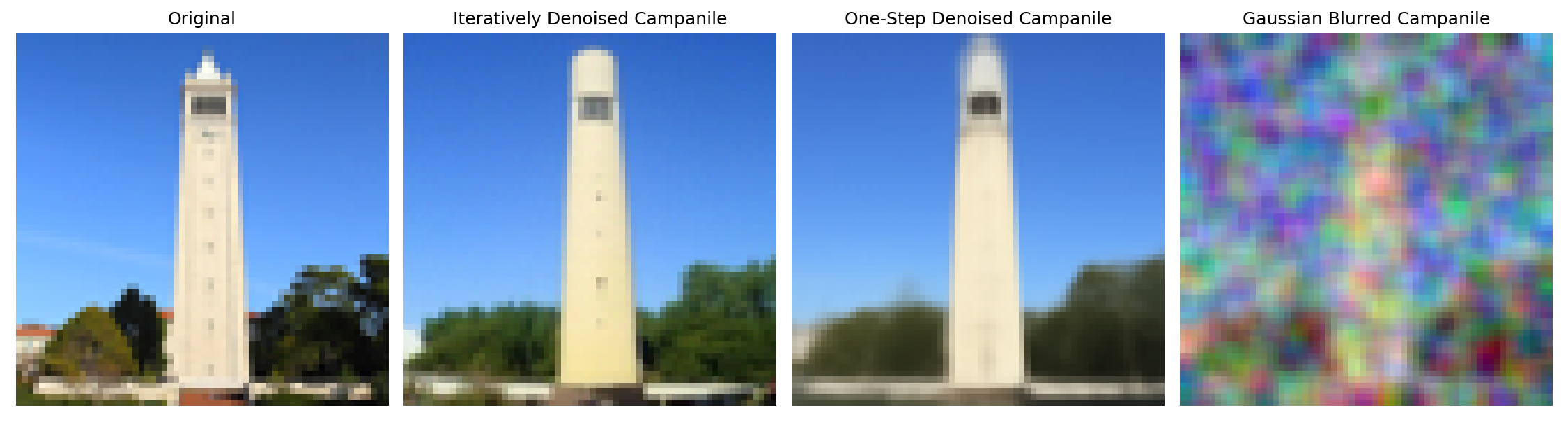
i_start = 10 (seed = 100)
A.1.5: Diffusion Model Sampling
Diffusion models can not only denoise images, but also able to
generate new images from scratch by starting from pure noise, i.e.,
setting i_start = 0 and passing random noise as our
im_noisy to our
iterative_denoise function. Recall that DeepFloyd
requires text conditioning as input, here we use a neutral prompt "a
high quality photo" again.
Implementation & Results
To sample images from scratch, we can generate random noise of shape
$(1,3,64,64)$ via
im_noisy = torch.randn(1, 3, 64, 64).half().to(device),
and pass it to our iterative_denoise function with
i_start = 0 and embedding of the neutral prompt. For
reproducibility purposes, I sample images with
seeds = [0, 1, 3, 4, 5], each of which produces a
distinct image as shown below.
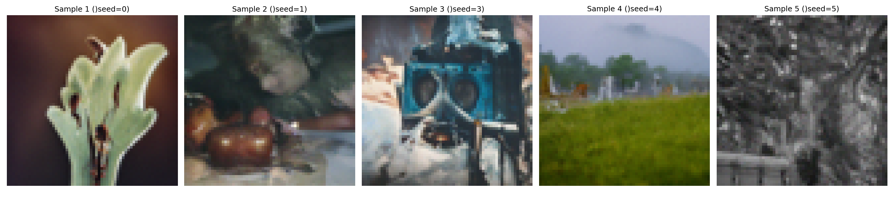
seeds = [0,1,3,4,5]
Obviously, the sampled images are of high quality and look like real photos, hence, they lie on the natural image manifold somehow. However, some of them still look a bit strange and unnatural. We will fix this issue in the next part with Classifier-Free Guidance!
A.1.6: Classifier-Free Guidance
As we noticed in the previous part that some of the generated images are not very good and even completely non-sensical, here we improve the quality (at the expense of image diversity) with a technique called Classifier-Free Guidance (CFG), where we compute both a conditional ($\epsilon_c$) and an unconditional ($\epsilon_u$) noise to get our new noise estimate through: $$ \epsilon = \epsilon_u + \gamma(\epsilon_c - \epsilon_u),\tag{A.4} $$ where $\gamma$ controls the strength of CFG. From the equation, we can see that $\gamma=0$ corresponds to an unconditional noise estimate, and $\gamma=1$ corresponds to a conditional noise estimate. By setting $\gamma > 1$, we can push the noise estimate further towards the conditional direction, which encourages the model to generate images that better align with the text prompt, hence improving quality. More details can be found in this blog post.
In practice, the "unconditional" embedding corresponds to an empty prompt, i.e., ""(nothing is in the middle). Then, our previous "a high quality photo" prompt becomes a condition, even though it is still weak and neutral. We will use CFG with $\gamma=7$ all throughout all Part A experiments starting from here.
Implementation & Results
Implementation of CFG (iterative_denoise_cfg) is
straightforward, we just need to modify our previous
iterative_denoise function to compute both conditional
and unconditional noise estimates, and combine them via equation
(4). With CFG, let's again sample some images from scratch and see
how it improves the quality. Here I picked
seeds = [0, 2, 3, 4, 5] and set scale = 7.
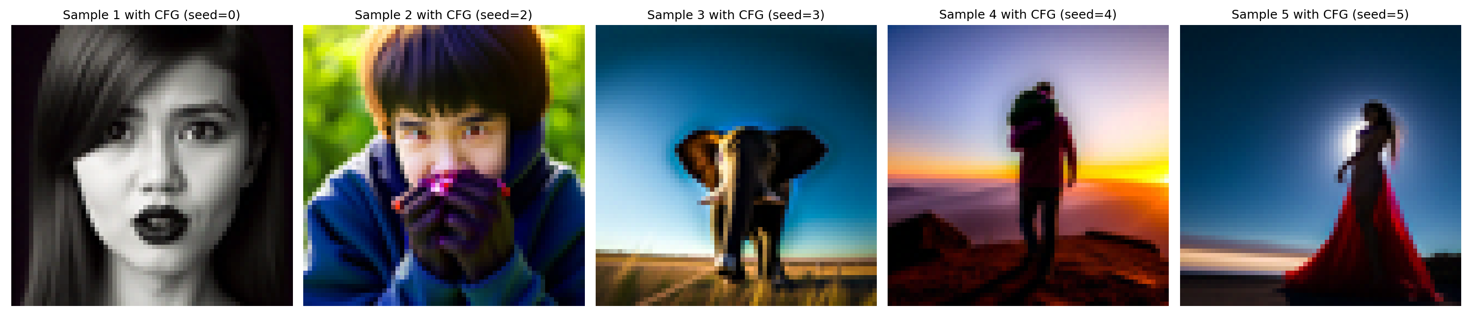
seeds = [0,2,3,4,5],
scale = 7
The results above look much better than those without CFG, all of which now look like real photos and nothing non-sensical!
A.1.7: Image-to-image Translation
The diffusion model can also be used to edit images, as we already saw in part 1.4 when we add noise to an image and then denoise it, where the reconstructed images were different from the original one. This works because the diffusion model has to "hallucinate" new things to fill in the missing details in the noised image, hence, the model has to be "creative" and force the noisy image back onto the manifold of natural images during denoising.
Here, we will follow the
SDEdit algorithm
to perform such image-to-image translation. The idea is we first add
some noise to the original image (by forward), and then
denoise it back with the diffusion model without extra text
conditioning (i.e., via
iterative_denoise_cfg conditioned on "a high quality
photo"). The reconstructed image then becomes an edited version of
the original image, which may look like the original image, but with
some details "edited".
Implementation & Results
Conditioned on the prompt "a high quality photo" and with CFG scale
of 7, here we edit the Campanile image and 2 cat images at noise
levels of i_start = [1, 3, 5, 7, 10, 20]. Since the
higher i_start, the less noise is added, hence, the
edited image will look more similar to the original image. The
results are shown below.
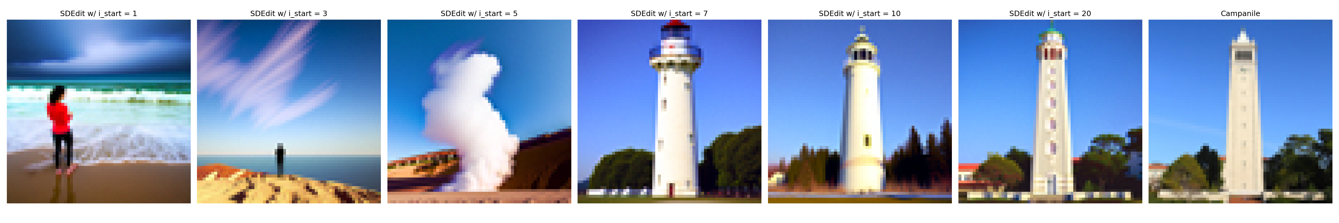
i_start = [1,3,5,7,10,20] (seed = 100)
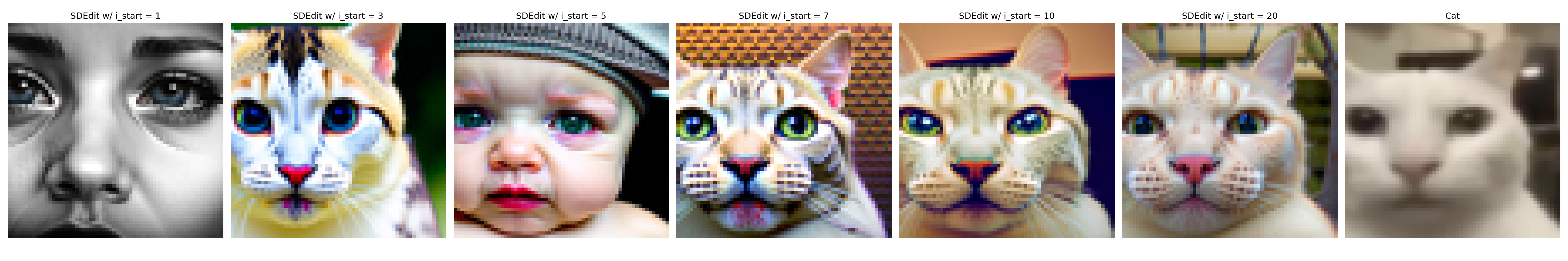
i_start = [1,3,5,7,10,20] (seed = 100)
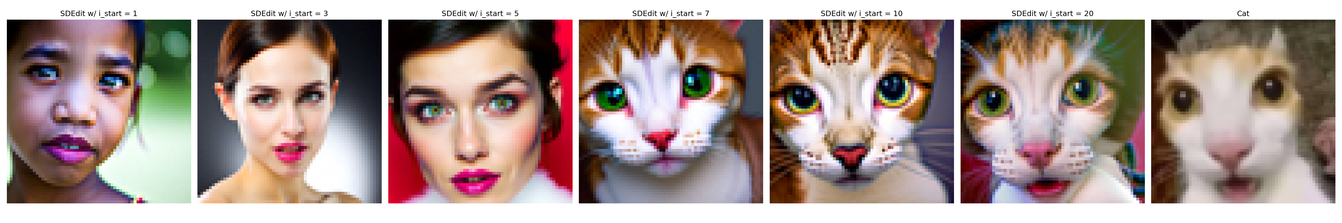
i_start = [1,3,5,7,10,20] (seed = 100)
A.1.7.1: Editing Hand-Drawn and Web Images
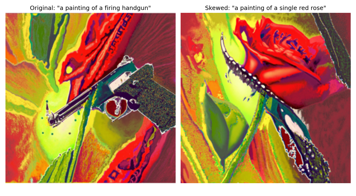
This SDEdit approach works particularly well for starting from nonrealistic images (e.g., paintings, sketches, some scribbles) and project them onto the natural image manifold.
Implementation & Results
Let's try applying the same procedure on one web image (a rose) and two of my hand-drawings created in Procreate (the Campanile and a panda). Everything is the same as in Part A.1.7, except that the starting images are different. The results are shown below.
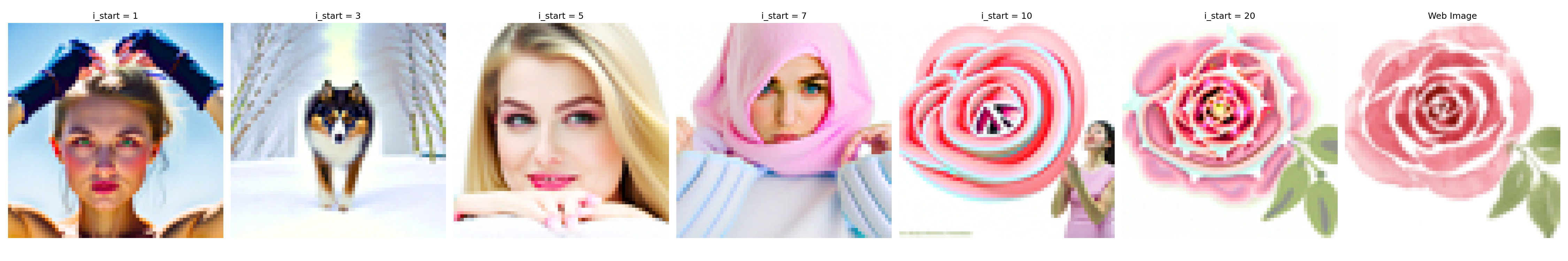
i_start = [1,3,5,7,10,20] (seed = 100)
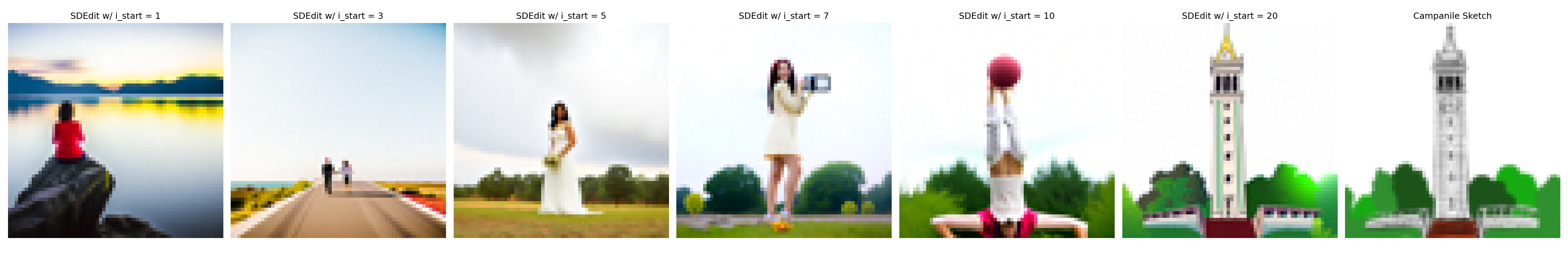
i_start = [1,3,5,7,10,20] (seed = 100)
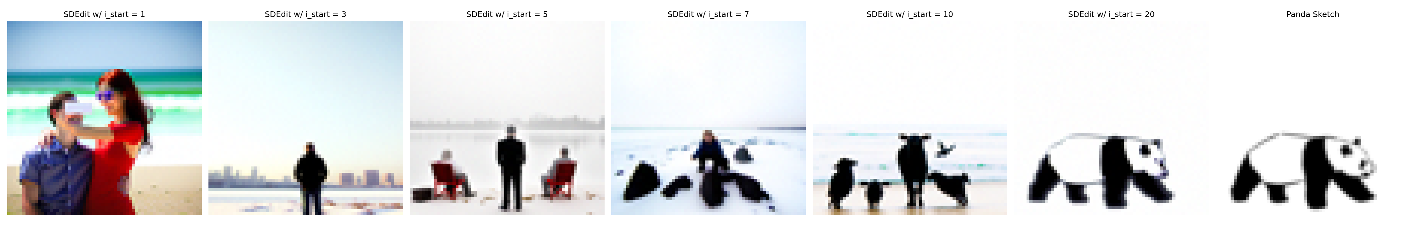
i_start = [1,3,5,7,10,20] (seed = 100)
It can be observed that adding little noise (e.g.,
i_start = 20) helps to refine the images while
preventing most of the original structure from being lost, while
adding more noise will yield somewhat the same general structure but
quite different details. However, if we add too much noise, the
results will be off the original image (particularly when
i_start = [1, 3]) too much, even not have a similar
structure.
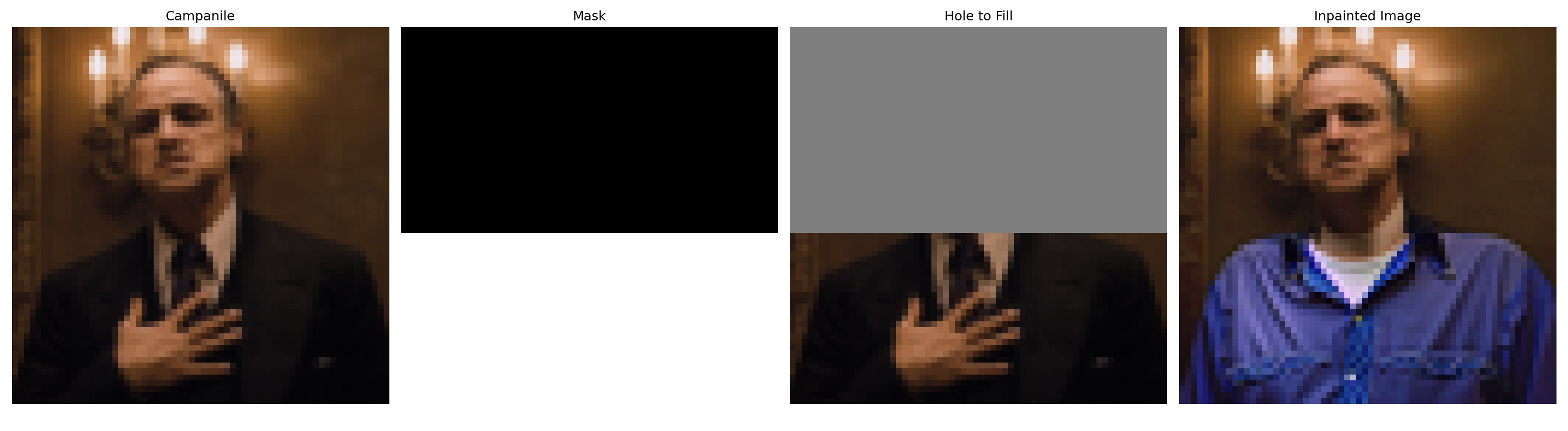
A.1.7.2: Inpainting
We can also use the same procedure to perform image inpainting (following the RePaint paper). The inpainting process uses a binary mask $\mathbf{m}$ and applies it to the original image $x_{orig}$, and creates a new image that has the same content where $\mathbf{m} = 0$ and new content where $\mathbf{m} = 1$. This can be achieved by "forcing" the obtained $x_t$ at every step in the denoising loop to have the same pixels as $x_{orig}$ where $\mathbf{m} = 0$, i.e, $$ x_t \gets \mathbf{m} x_t + (1 - \mathbf{m}) \texttt{forward}(x_{orig},t).\tag{A.5}$$
Implementation & Results
The implementation of the inpaint function can be
easily obtained by simply modifying the denoising loop in
iterative_denoise_cfg to apply the mask at every step.
With the implemented function, let's try inpainting on the Campanile
and 2 of my own images. For better results, I tried multiple seeds
and picked the one that looks interesting to myself.
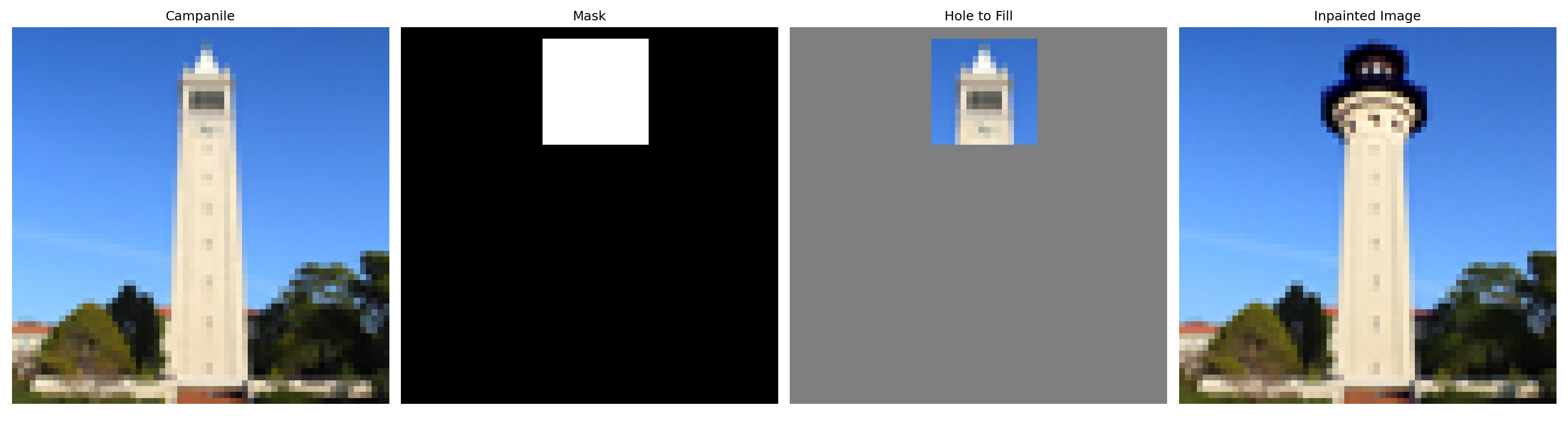
i_start = [1,3,5,7,10,20] (seed = 38)
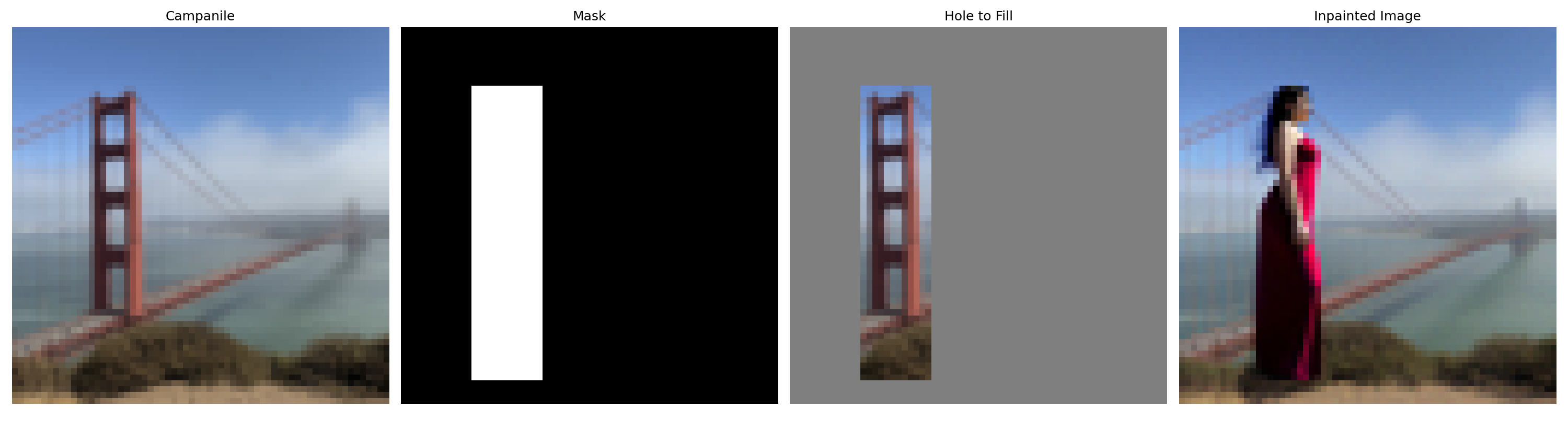
i_start = [1,3,5,7,10,20] (seed = 14)
i_start = [1,3,5,7,10,20] (seed = 17)
A.1.7.3: Text-Conditional Image-to-image Translation
Instead of conditioning on a neutral prompt, we can also perform SDEdit guided by a specific text prompt, which no longer acts as a pure “projection” onto the natural image manifold, but adds controllability through language.
Implementation & Results
Let's do the text-conditional SDEdit on the Campanile and two of my
selected images. With the increase of i_start, the
edited images look more similar to the original images, while still
incorporating elements from the text prompts. The prompts are shown
in the captions
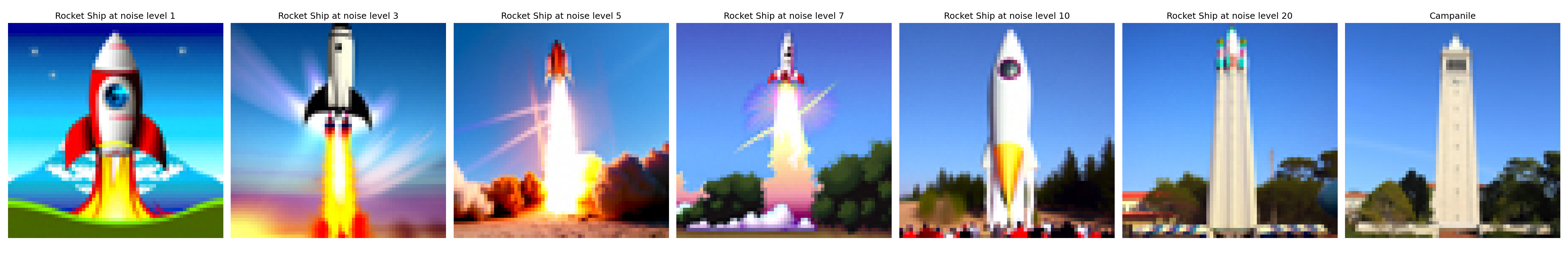
i_start = [1,3,5,7,10,20] (seed = 100), prompt = "a
rocket ship"
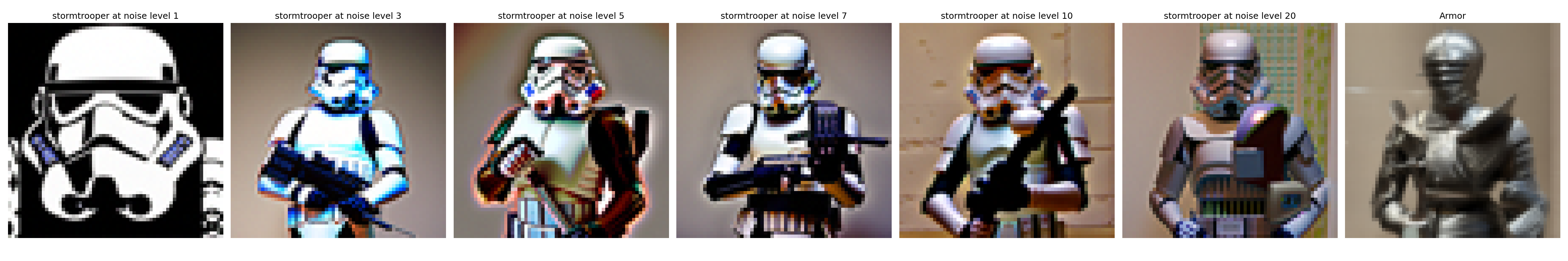
i_start = [1,3,5,7,10,20] (seed = 100), prompt = "a
stormtrooper from Star Wars"
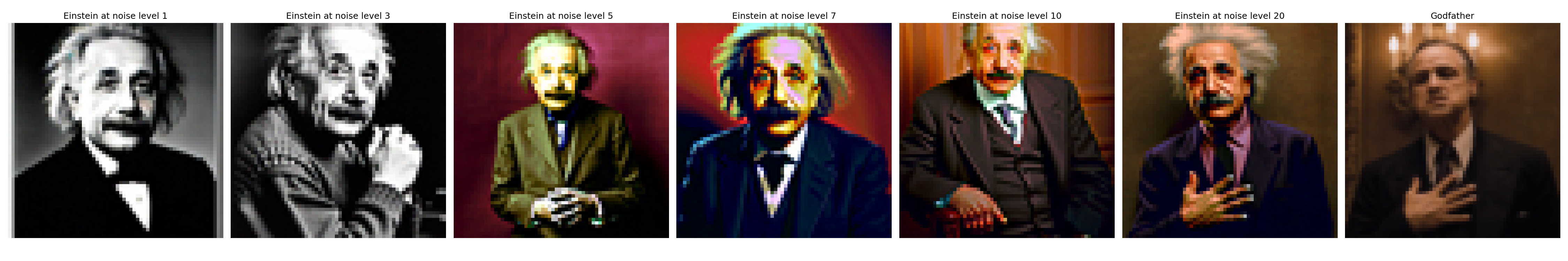
i_start = [1,3,5,7,10,20] (seed = 100), prompt =
"Albert Einstein"
A.1.8: Visual Anagrams
In this part, we will implement the Visual Anagrams and create optical illusions with diffusion models. The idea is to generate an image that can be interpreted in two different ways before and after some orthogonal transformations (e.g., flipping, rotation, etc.).
To achieve this, we will denoise an image $x_t$ at step $t$ normally with the prompt $p_1$, to obtain noise estimate $\epsilon_1$. But at the same time, we will apply the orthogonal transformation to $x_t$ and denoise with the prompt $p_2$ to get noise estimate $\epsilon_2$, after which, we transform $\epsilon_2$ back to the original orientation. Finally, we can perform a reverse/denoising step with the averaged noise estimate. The full algorithm is: $$\epsilon_1 = \text{CFG of UNet}(x_t, t, p_1),\tag{A.6}$$ $$\epsilon_2 = \text{transform_back}(\text{CFG of UNet} (\text{transform}(x_t), t, p_2)),\tag{A.7}$$ $$\epsilon = (\epsilon_1 + \epsilon_2) / 2,\tag{A.8}$$ where the UNet is the diffusion model UNet from before, $\text{transform}(\cdot)$ is the orthogonal transformation function and $\text{transform_back}(\cdot)$ is its inverse, and $p_1$ and $p_2$ are two different text prompt embeddings, and $\epsilon$ is our final noise estimate.
Implementation & Results
There are multiple orthogonal transformations we can use, here I
first used the $\text{flip}(\cdot)$ function that flips the image
both horizontally and vertically, i.e., a 180-degree rotation. Two
example visual anagrams created with the flip function are shown
below. In both cases, the images can be interpreted as different
scenes before and after a 180-degree rotation (animated as follows).
They are sampled with seed = 28 and
seed = 2, respectively.
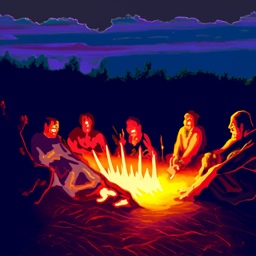
an oil painting of people around a campfire
a photo of a volcano
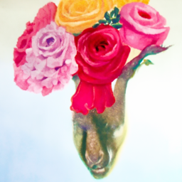
a watercolor painting of flower arrangements
a photo of a dress
A.1.9: Hybrid Images
From part A.1.8, we can see that playing with the noise estimates at each step can yield interesting visual illusions, such as visual anagrams through orthogonal transformations. Not limited in orthogonal transformations, here we will implement Factorized Diffusion and create hybrid images similar to those in project 2, i.e., images whose interpretation changes as a function of viewing distance.
To do this, we will follow almost the same procedure as in part A.1.8 but applying low- and high- pass filters to the two noise estimates respectively before fusing them via sum. The algorithm is as follows: $$\epsilon_1 = \text{CFG of UNet}(x_t, t, p_1),\tag{A.9}$$ $$\epsilon_2 = \text{CFG of UNet}(x_t, t, p_2),\tag{A.10}$$ $$\epsilon = f_{\text{lowpass}}(\epsilon_1) + f_{\text{highpass}}(\epsilon_2)\tag{A.11}.$$
Implementation & Results
In my implementation, I use Gaussian filters for both low- and
high-pass filtering, with a kernel_size = 33 and
sigma = 2 for the low-pass filter. Two example hybrid
images are shown and animated below. They are generated with
seed = 8 and seed = 36, respectively, and
can be interpreted as different scenes when viewed up close versus
from afar.
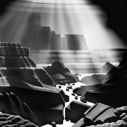
a photo of grand canyon
Albert Einstein
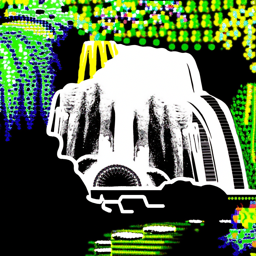
a lightgraph of waterfalls
a photo of a panda
B & W: More visual anagrams!
There are much more orthogonal transformations that can be used to create visual anagrams. Here let's implement two more!
1. Approximated Skew Anagram
Here I will implement the skew transformation to create visual anagrams. Since the true skew transformation that inplemented via homography is not "orthogonal" as it relies on interpolation, we instead implement an approximated version mentioned in the paper, i.e., skewing by columns of pixels by different displacements. This column-roll skew preserves pixel values and acts as a permutation matrix, thus satisfying the orthogonality constraint required by the noise-preserving property of diffusion models.
Implementation & Results
The implementation of this approximated skew transformation is straightforward once we have our previous flip anagram code, i.e., just replace the flip operation with the skew operation. Here I'm showing the skew operation code snippet below.
Code Snippet:
implement skew operation in
make_skew_illusion
def skew_img(img, max_disp):
    b, c, h, w = img.shape
    # shifts for each column
    shifts = torch.linspace(-max_disp, max_disp, steps=w, device=img.device).round().long()  # (w,)
    # raw row indices of all pixels
    row_idx = torch.arange(h, device=img.device).view(h, 1) # (h, 1)
    # shifted row indices
    shifted_row_idx = (row_idx - shifts) % h # (h, w)
    shifted_row_idx = shifted_row_idx.view(1, 1, h, w).expand(b, c, h, w) # (b, c, h, w)
    # gather all pixels for skewed image
    skewed_img = torch.gather(img, 2, shifted_row_idx)
    return skewed_img
To use it, we just need to defined a max_disp as our
maximum column displacement (in pixels) as an extra argument to the
illusion function, then call the above
skew_img(im, max_disp) as our transformation, and
skew_img(im, -max_disp) as its inverse. The results of
one example skew anagrams are shown below, with
max_disp = 50 on a $64 \times 64$ image. The image was
sampled with seed = 82.
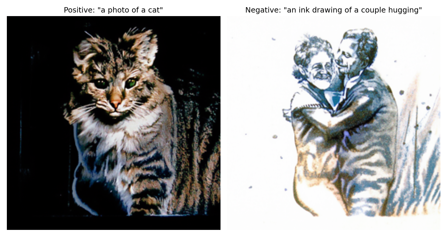
2. Negative Anagram
Not limited to geometric permutations, the color inversion like negatives can also be used as the orthogonal transformation, as it is intuitively a $180$ degree rotation generalized to higher dimensions, which allows us to generate illusions that change appearance upon color inversion, assuming pixel values are centered at $0$ (i.e., in $[-1, 1]$ range). Here we implement such negative anagram.
Implementation & Results
The implementation of negative anagram is even simpler. Everything
is the same as our flip anagram code, except that the transformation
function now is negative_img, defined as below, whose
forward and inverse operations are the same.
Code Snippet:
implement negative operation in
make_negative_illusion
def negative_img(img):
    return -img
One example negative anagram is shown below. The image was sampled
with seed = 68. (Note: To be honest, this negative
anagram is so good and was out of my expectations, I couldn't even
tell the opposite interpretation before taking the negatives of each
of them!)
The following animation shows how the negative anagram changes appearance upon color inversion.
B & W: Design a course logo!
I wanted to create a logo that a bear hidding behind a filter filled with some features of UC Berkeley. To do so, I sketched such a bear in Procreate, and filling the $3 \times 3$ kernel with colors representing UC Berkeley. The original sketch is shown below.
Then, I used this sketch as the input image to perform
text-conditional image-to-image translation to refine it. The prompt
I used was "A clean, minimalistic course logo of the computer vision
course of the University of California at Berkeley. A cute cartoon
bear peeks from behind a square sign. Inside the square is a simple
3x3 convolution kernel diagram. Smooth bold outlines, flat look,
friendly style". Then, with seed = 9,
i_start = 25 and scale = 7, I obtained the
final logo as shown below, which, although it somehow changed the
original color but looks more professional and appealing, at least
aligns my expectation :D.
Part B: Flow Matching from Scratch!
As we have explored diffusion models extensively in part A, now let's dive into flow matching models and implement our own for image generation from scratch! Again, the implementation will follow this provided notebook, and we will play with MNIST dataset for simplicity.
B.1: Training a Single-Step Denoising UNet
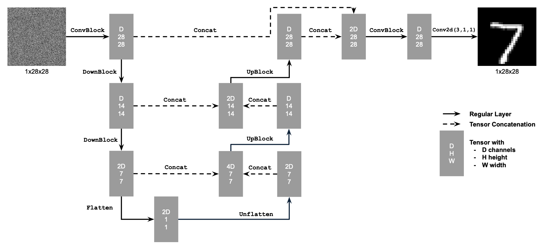
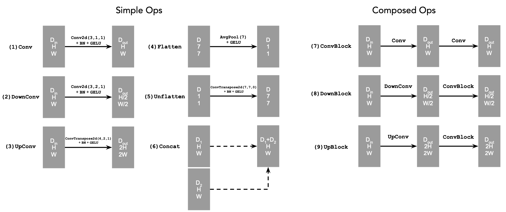
B.1.1: Implementing the UNet
In this whole part B, we will implement and use UNet as our backbone for denoising and flow matching, i.e., the $D_{\theta}$. This architecture encodes the input image into a latent representation and then decodes it back to the original image space, while incorporating skip connections to preserve both low and high frequency spatial information. The implemented UNet follows the architecture shown in the figure below, including its architecture details and atomic operations.
B.1.2: Using the UNet to Train a Denoiser
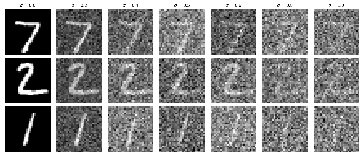
Here we first train the $D_{\theta}$ as a one-step denoiser, i.e., predicting the clean image $x$ from a noisy input $z$ directly, which can be done by minimizing the $\mathcal{L}_2$ loss mentioned in equation (B.1) above. The clean images are sampled from the MNIST training set ($x \sim \mathcal{D}_{\text{MNIST}}$), and the noise image $z$ is generated by adding Gaussian noise to $x$: $$z = x + \sigma \epsilon, \quad\text{where}\,\, \epsilon \sim \mathcal{N}(0, \mathbf{I}),\tag{B.2}$$ where the $\sigma$ controls the noise level.
Visualization of the Noising Process
The visualization of the noising process with $\sigma = [0.0, 0.2, 0.4, 0.5, 0.6, 0.8, 1.0]$ is shown below.
B1.2.1 Training
We can now train our UNet denoiser to denoise the noisy images $z$ generated by $\sigma=0.5$ from clean images $x$. The model is created following the architecture shown in B.1.1, optimized by Adam, and the hyperparameters are summarized in the following table.
batch_size |
learning_rate |
noise_level |
hidden_dim |
num_epochs |
|---|---|---|---|---|
| 256 | 1e-4 | 0.5 | 128 | 5 |
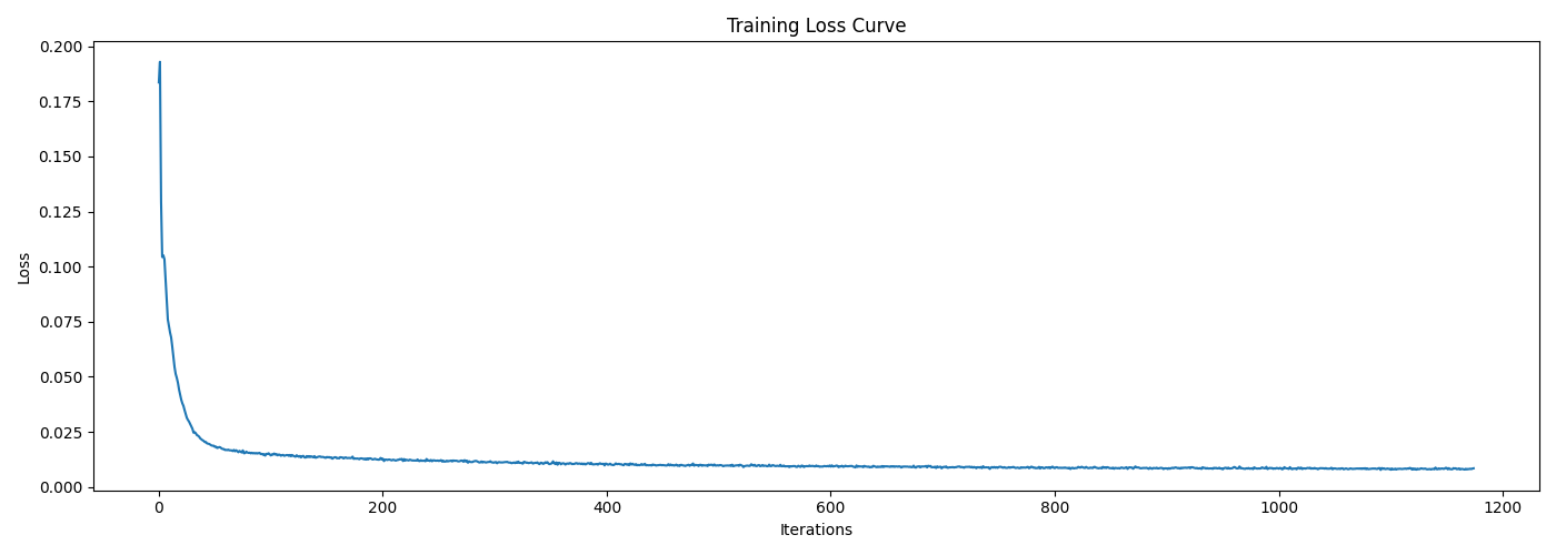
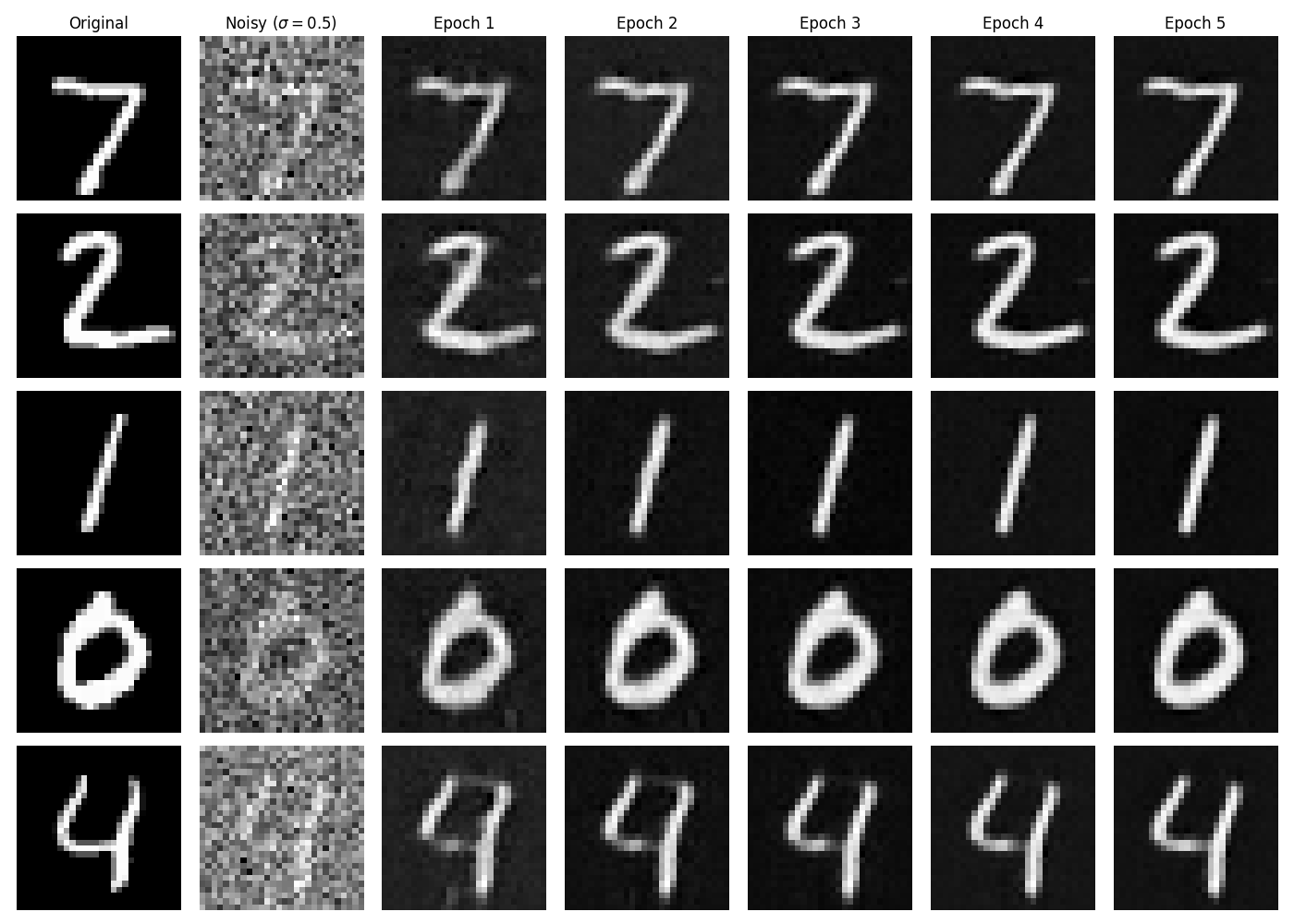
Training Curve & Sample Results
The training loss curve is shown below, indicating that the model converges very fast and stably. Setting the same level of noise ($\sigma=0.5$), the denoised results on some test samples after checkpointing the model at different epochs are shown as well.
B1.2.2 Out-of-Distribution Testing
Our denoiser was trained on fixed noise level $\sigma=0.5$. Here we test its generalization on other noise levels. The denoised results on noisy test samples with $\sigma = [0.0, 0.2, 0.4, 0.5, 0.6, 0.8, 1.0]$ are shown as follows.
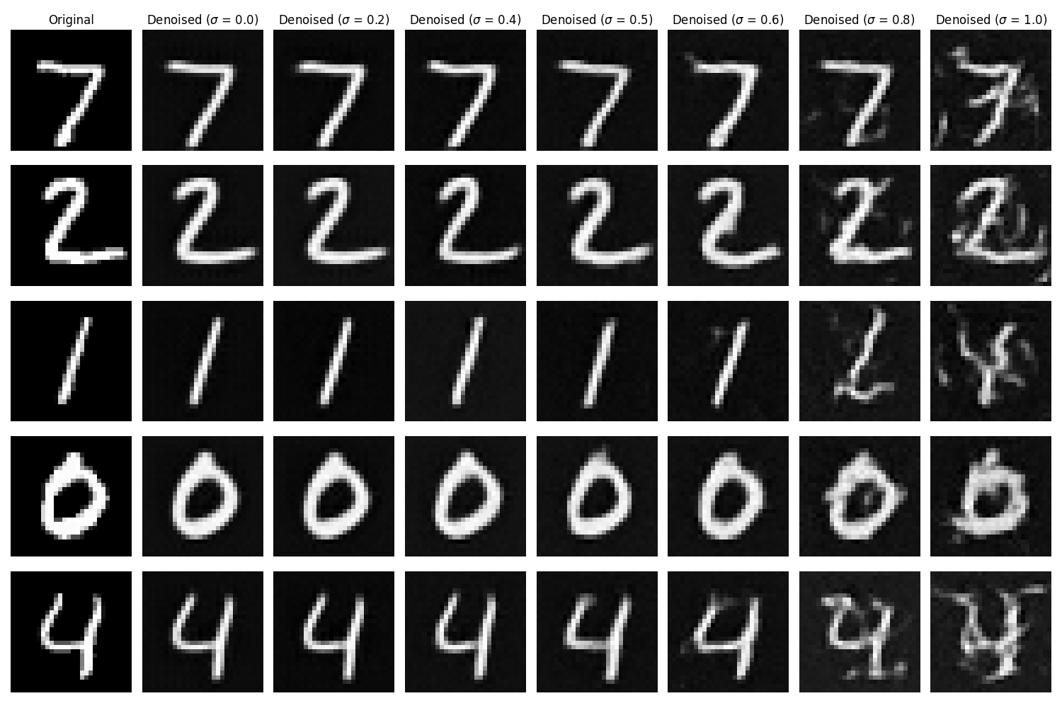
It is obvious that the denoiser performs well on noise levels close to or lower than the training level, while it gradually degrades when denoising on higher levels, which is expected as it did not learned to handle such highly noisy cases during training.
B1.2.3 Denoising Pure Noise
Recall that to make the denoising model generative, as discussed in Part A, we can apply to denoise pure noise, hence, $z = \epsilon \sim \mathcal{N}(0, \mathbf{I})$ as input, instead of being generated from $x$ anymore. Now, let's try this with our one-step UNet denoiser. Here we follow exactly the same procedure as in B.1.2.1 to train a UNet, where the only change is that $z = \epsilon \sim \mathcal{N}(0, \mathbf{I})$ as our input.
Results & Discussion
The training loss curve and some sampled denoised results from pure noise after different epochs are shown below.
It can be observed that all generated images sampled from pure noise look almost identical. This is because the input distribution $Z \sim \mathcal{N} (0, \mathbf{I})$ provides no additional information as the condition for the model to generate diverse outputs in the target distribution $X \sim \mathcal{D}_{\text{MNIST}}$, hence, we have $Z \perp X$.
Ideally, if we train a model with the following MSE loss function: $$\mathcal{L} = \mathbb{E}_{Z, X} \left[ \| D_{\theta}(z) - x \|^2 \right],$$ the optimal solution should be the conditional expectation of $X$ given $Z$: $$D_{\theta}^*(z) = \mathbb{E}[X|Z].$$
However, since the independence between $Z$ and $X$ holds, we have: $$\mathbb{E}[X|Z] = \mathbb{E}[X].$$
Therefore, the denoiser is a constant function for $Z$ that always outputs the mean of the target distribution $\mathbb{E}[X]$, i.e., $$D_{\theta}^*(z): Z \to \mathbb{E}[X]\quad$$
Since the MNIST digits are centered around the middle of the image and are in the same scale, the mean of the target distribution is a weighted average of all digits, where the shared pattern will be highlighted, resulting in the image shown above.
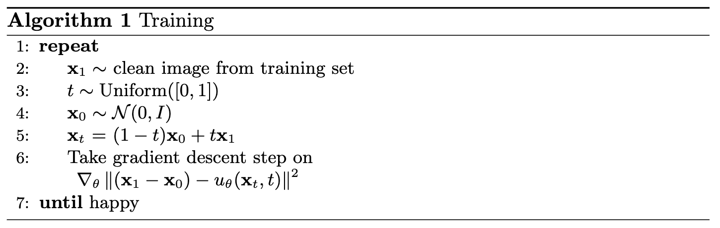
B.2: Training a Flow Matching Model
We just saw that one-step denoising from pure noise fails to generate diverse new samples due to the limitation of the training objective. Instead, we need to gradually denoise from pure noise to data through multiple steps, like what we did in Part A with diffusion models. Here, we will do so via flow matching, where our UNet model will learn to predict the "flow" that transports noise to the clean data manifold over continuous time, i.e., an ordinary differential equation (ODE) describing the transformation from noise to data. Then, in the sampling stage, we can solve this ODE to generate a new realistic image $x_1$ from pure noise $x_0 \sim \mathcal{N}(0, \mathbf{I}).$
For iterative denoising, we need to define how intermediate noisy samples are constructed, where the simplest approach is the linear interpolation between noise and data in our training set: $$x_t = (1-t)x_0 + t x_1 \quad \text{where}\,\, x_0 \sim \mathcal{N}(0, \mathbf{I}), \,\, t \in [0,1].\tag{B.3}$$
This is a vector field describing the position of a point $x_t$ at time $t$ relative to the clean data distribution $p_1(x_1)$ and the noisy data distribution $p_0(x_0)$. Ituitively, we see that for small $t$, we remain close to noise, while for larger $t$, we approach the clean distribution.
The "flow" can be interpreted as the velocity of this vector field that describing how points move from noise to data over time, i.e., $$u(x_t,t) = \frac{d}{d t} x_t = x_1 - x_0.\tag{B.4}$$
Therefore, our aim is to learn a $u_{\theta}(x_t, t)$ with our UNet model that approximates this flow $u(x_t, t) = x_1 - x_0$ through the objective below: $$ \mathcal{L}(\theta) = \mathbb{E}_{x_0 \sim p_0(x_0), x_1 \sim p_1(x_1), t\sim \text{Unif}(0,1)} \left[ \|(x_1 - x_0) - u_{\theta}(x_t, t)\|^2_2 \right].\tag{B.5}$$
B.2.1 Adding Time Conditioning to UNet
Since our flow matching model $u_{\theta}(x_t, t)$ now takes an extra time variable $t$ as input, we need to modify our previous UNet architecture to condition it on $t$. There are many ways to do this, and we will follow the one introduced below.
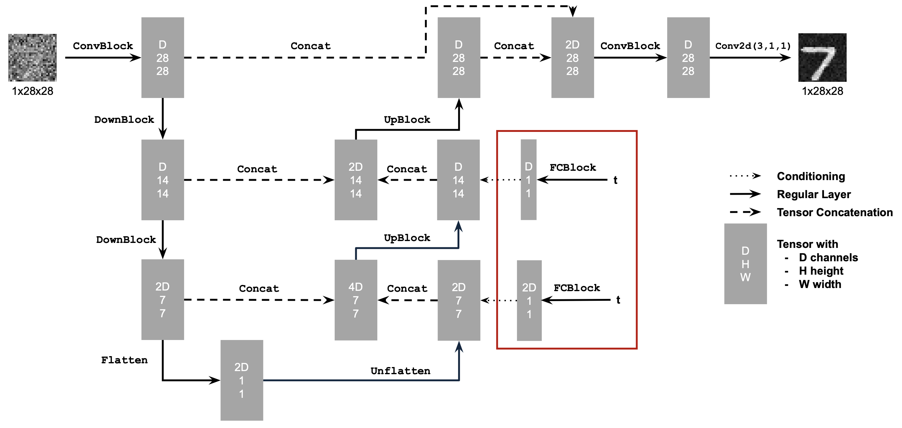
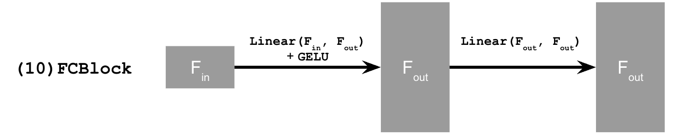
The new operator FCBlock is designed to encode and
inject the conditioning signals into the UNet.
With aforementioned new architectural design, our UNet can be conditioned on $t$ through the following pseudo-code:
Code Snippet: Time conditioning in UNet on t
fc1_t = FCBlock(...)
fc2_t = FCBlock(...)

# the t passed in here should be normalized to be in the range [0, 1]
t1 = fc1_t(t)
t2 = fc2_t(t)

# Follow diagram to get unflatten.
# Replace the original unflatten with modulated unflatten.
unflatten = unflatten * t1
# Follow diagram to get up1.
...
# Replace the original up1 with modulated up1.
up1 = up1 * t2
# Follow diagram to get the output.
...
B.2.2 Training the Time-Conditioned UNet
The training of the time-conditioned UNet flow matching model follows the architecture introduced in B.2.1, trained on the objective in equation (B.5) via the Adam optimizer. The exponential learning rate scheduler is used, where the gamma was set to $0.1^{(1.0/\texttt{num_epochs})}$. Key hyperparameters are summarized in the following table.
batch_size |
learning_rate |
hidden_dim |
num_epochs |
|---|---|---|---|
| 64 | 1e-2 | 64 | 10 |
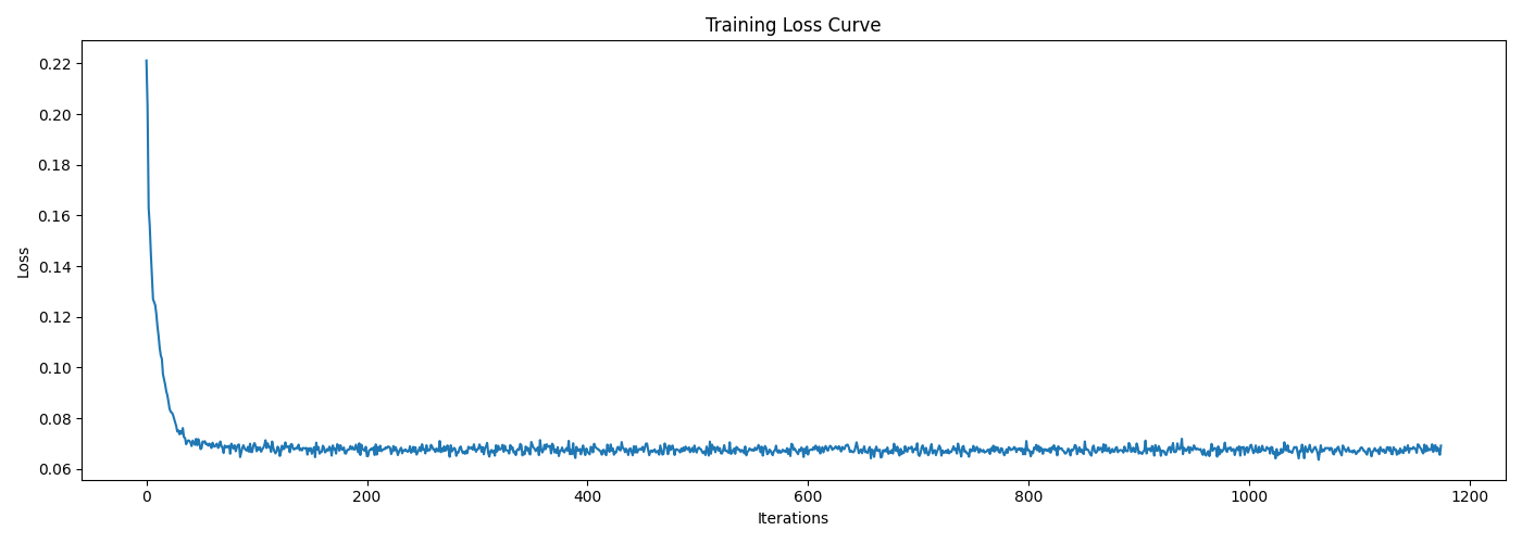
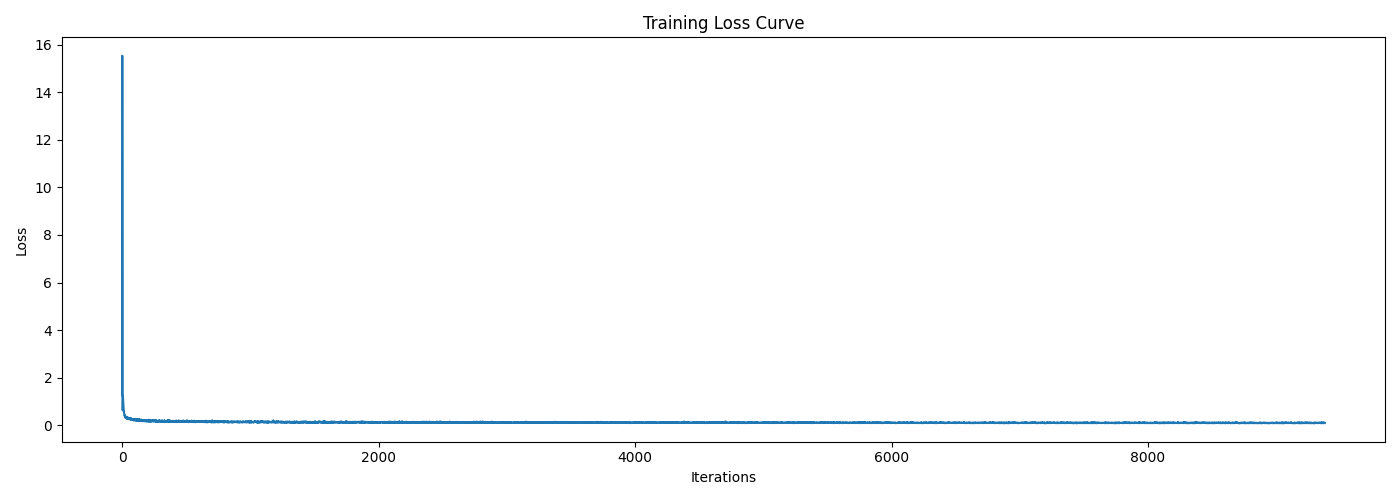
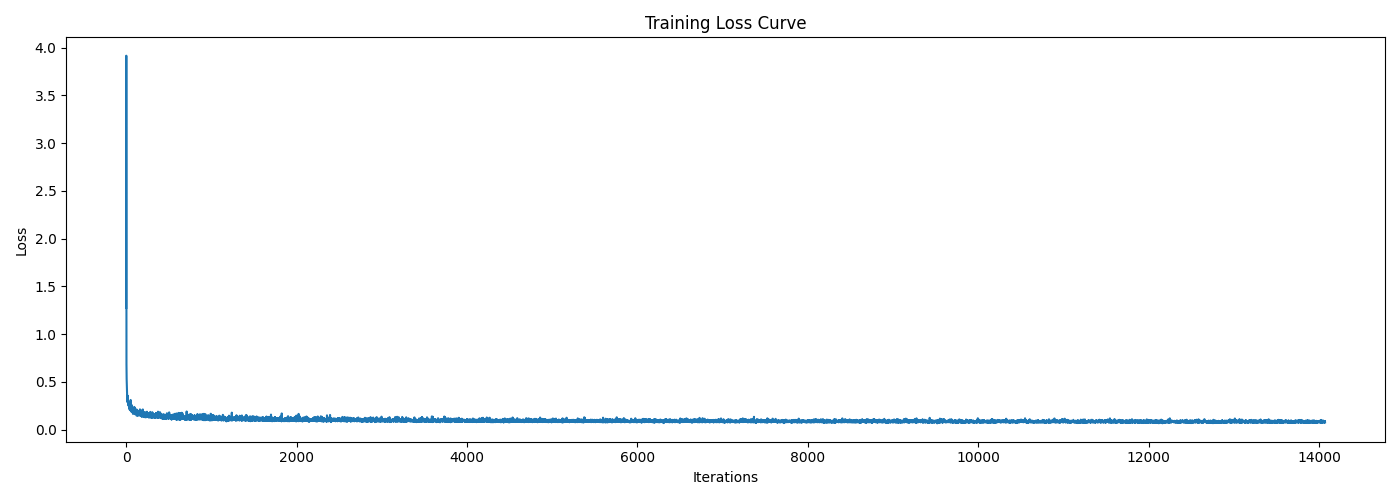
The training process follows Algorithm 1 shown below, and the training loss curve is also attached afterwards, where we can observe a sharp decrease at the beginning and then a stable convergence. The training process is quite fast, which is good for our implementation.
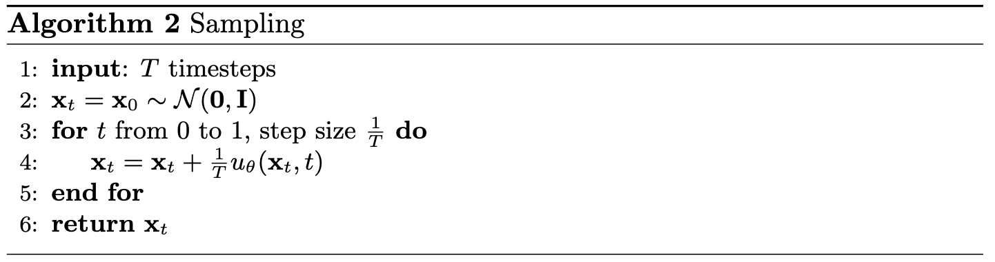
B.2.3 Sampling From the Time-Conditioned UNet
We can now sample new images from pure noise by iteratively solving the ODE defined by our trained UNet flow matching model. The sampling procedure follows Algorithm 2 shown below, which is a simple Euler method with fixed step size $1/T$, and here I set $T=50$.
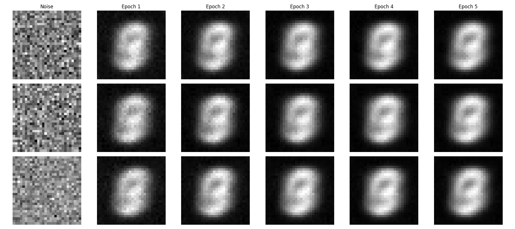
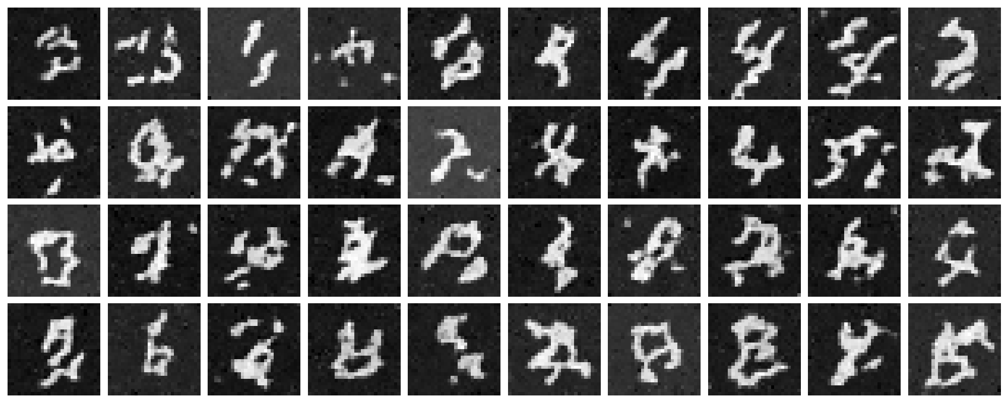
Sampling Results
The sampled new images at checkpoints of epochs $1$, $5$, and $10$ are shown below. It is obvious that the model gradually learns to generate more realistic and diverse digits as training proceeds. However, there are still some artifacts that make them far from perfect, though they are resonably good for only $10$ epochs of training. An improved version of this time-conditional only model can be found in the Bells & Whistles section in the end of this blog.
B.2.4 Adding Class-Conditioning to UNet
To make the results better and give us more control over the generation process, we can further condition our UNet model on class labels, i.e., the model now becomes $u_{\theta}(x, t, c)$ where $c$ is the class label.
In practice, we can add 2 more FCBlock to our UNet,
where the class conditioning vector $c$ will first be encoded as a
one-hot vector and then passed into these
FCBlock modules to be embeded and injected into the
UNet. To make our model able to work without being conditioned on
class labels, which is important to implement CFG during sampling,
we randomly drop the class conditioning vector $c$ to be an all-zero
vector with a probability of $10\%$ during training, hence,
$p_{uncond} = 0.1$. The peudo-code for conditioning our UNet on both
time and class labels is shown below.
Code Snippet: Time and class conditioning in UNet on t and c
fc1_t = FCBlock(...)
fc1_c = FCBlock(...)
fc2_t = FCBlock(...)
fc2_c = FCBlock(...)

t1 = fc1_t(t)
c1 = fc1_c(c)
t2 = fc2_t(t)
c2 = fc2_c(c)

# Follow diagram to get unflatten.
# Replace the original unflatten with modulated unflatten.
unflatten = c1 * unflatten + t1
# Follow diagram to get up1.
...
# Replace the original up1 with modulated up1.
up1 = c2 * up1 + t2
# Follow diagram to get the output.
...
B.2.5 Training the Class-Conditioned UNet
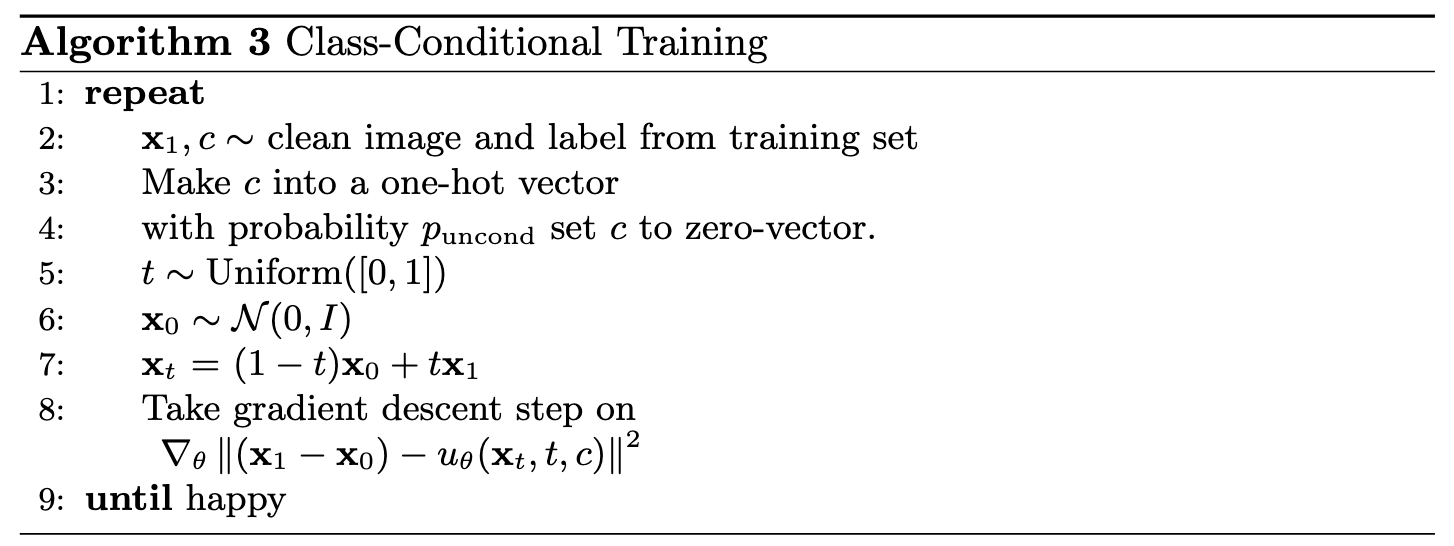
The training for this UNet with extra class conditioning follows almost the same procedure as the time-conditioned only one, where the only difference is to add the conditioning vector $c$ and do unconditional generation periodically, following Algorithm B.3 shown below.
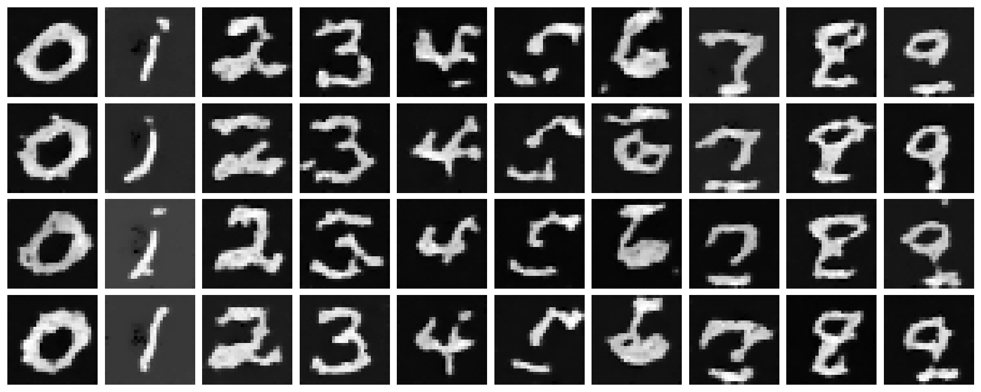
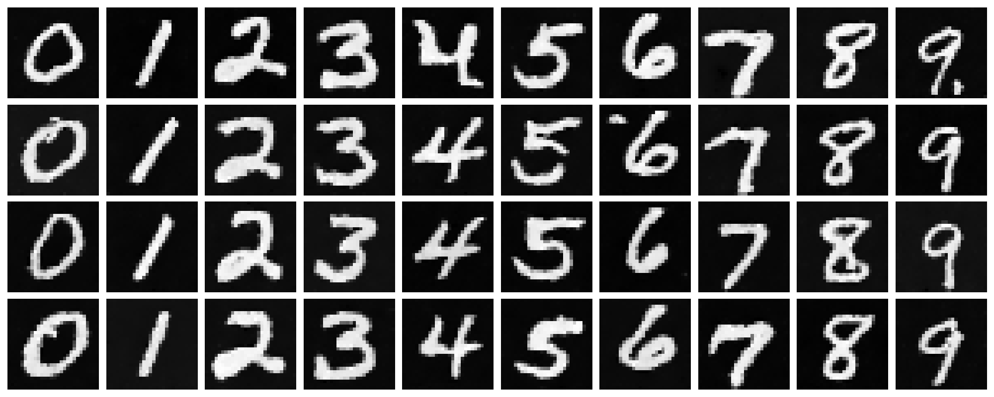
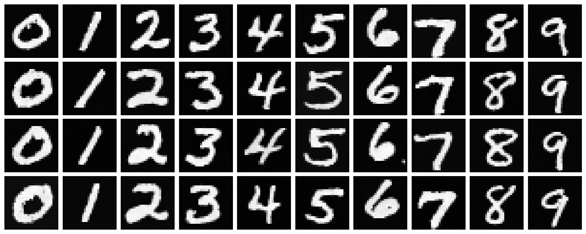
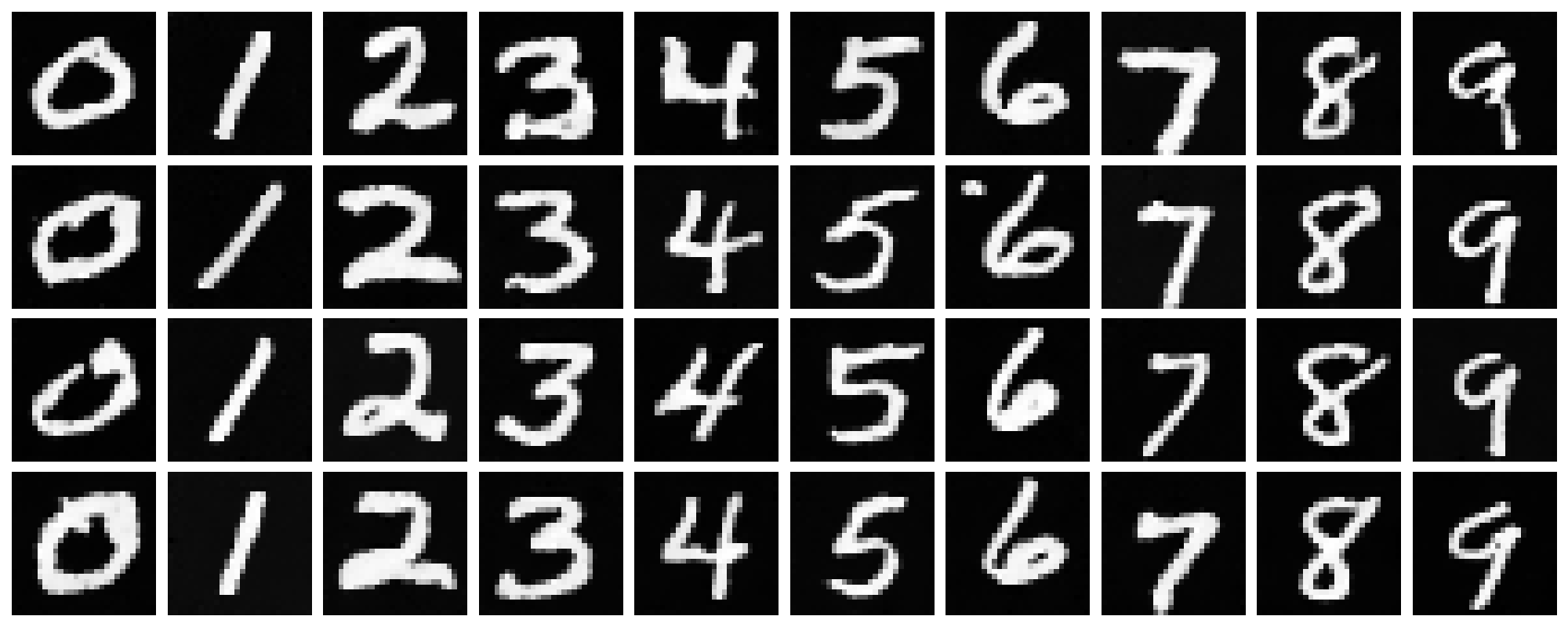
B.2.6 Sampling with Class-Conditioned UNet
We can now sample new images with our class-conditioned UNet flow matching model. With this class conditioning, we can further apply CFG during sampling to enhance the generation quality. The sampling procedure follows Algorithm B.4 shown below, where the guidance scale $\gamma$ is set to $5.0$ in my experiments.
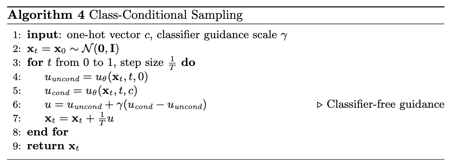
Sampling Results
The sampled new images at checkpoints of epochs $1$, $5$, and $10$ are shown below. It is obvious that the model generates more realistic digits with class conditioning and CFG, compared to the time-conditioned only model.
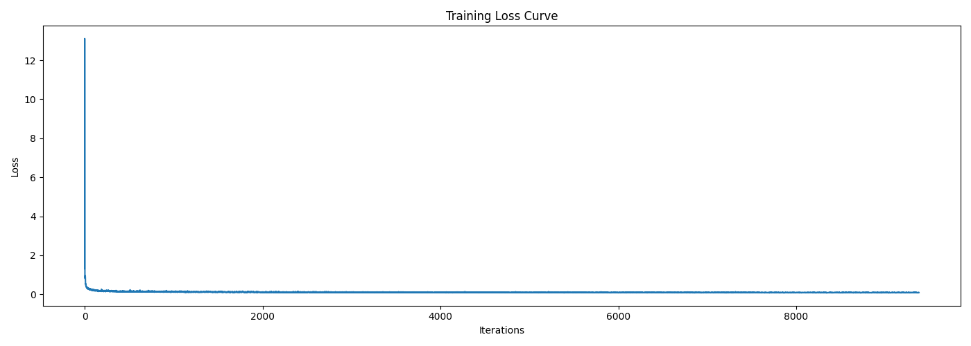
Getting Rid of Learning Rate Scheduler
Here comes a question: can we get rid of the annoying learning rate scheduler? The answer is yes! From the training loss curve above, we can see that the loss actually decreases quite quickly at the beginning, which indicates that the scheduler is actually not that necessary. Therefore, for simplicity, we can fix the learning rate to a smaller value, e.g., $5 \times 10^{-3}$, and train the model longer for $15$ epochs without the scheduler. The training loss curve for this new setting is shown below, which is quite similar to the previous one with the scheduler.
Also, let's sample some new images via this model at the last epoch and compare with the previous one with the scheduler, shown below. From the sampled results, I can not visually tell which one is better, meaning that fixing a smaller learning rate and training longer without the scheduler works just as well as using the scheduler.
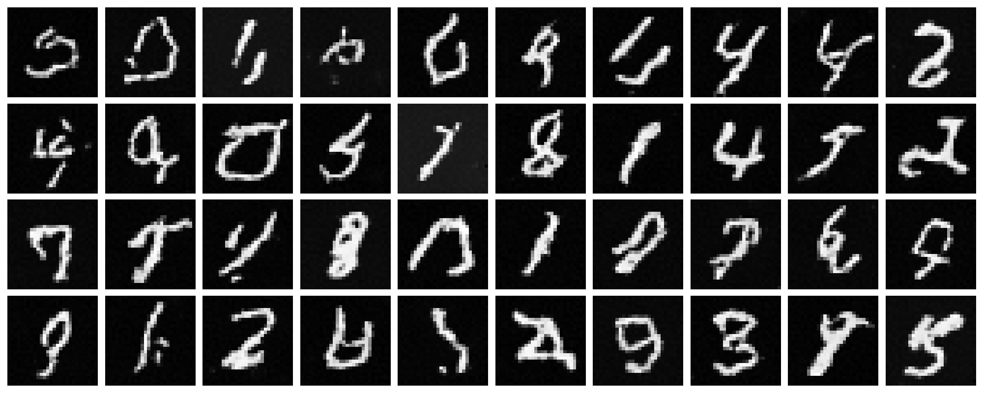
B & W: Better Time-Conditioned UNet
Recall that our time-conditioning only UNet in B.2.3 can even though generate digits from Gaussian noise, but the quality is not as good as the class-conditioned one, e.g., there are many artifacts making the digits hard to recognize. Therefore, here we try to improve it!
Since in this case we cannot apply CFG during sampling to enhance the generation quality, we instead enhance the model performance by improving its capacity of representation. For instance, here I increase the hidden dimension from $64$ to $128$. In the training stage, I also adjusted the initial learning rate to $5 \times 10^{-2}$, and increased the number of training epochs to $50$. The hyperparameters are summarized in the following table.
batch_size |
learning_rate |
hidden_dim |
num_epochs |
|---|---|---|---|
| 64 | 5e-2 | 128 | 50 |
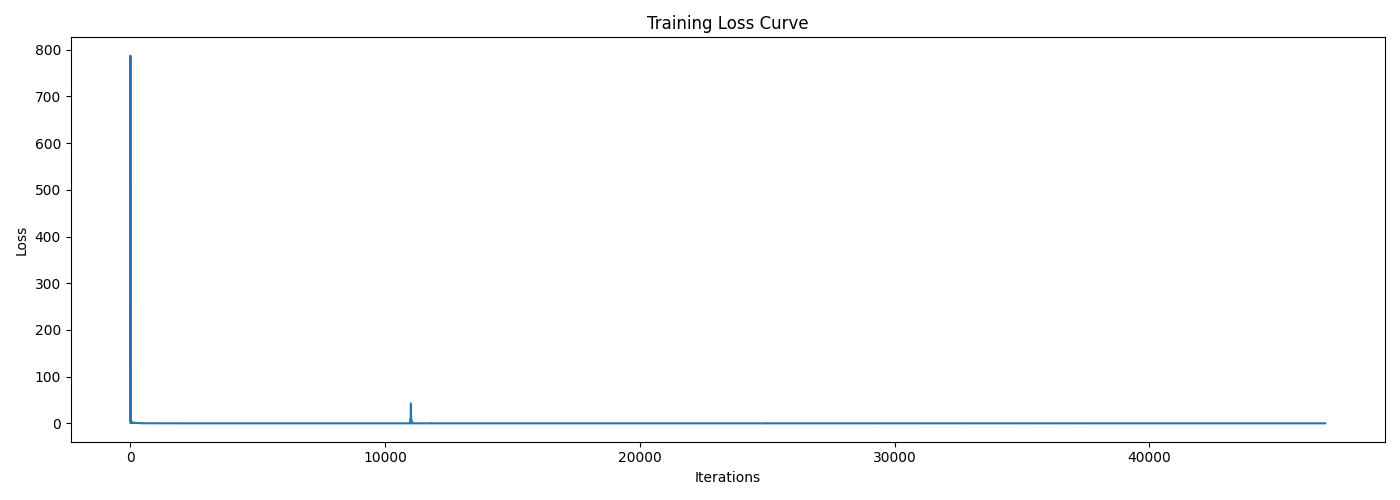
The training loss curve for this enhanced model is shown below, which indicates a quick and sharp reduction in loss at the beginning. Although we cannot directly see the convergence at later epoches due to the scale of the plot, we can still observe improvements in the sampled results shown later, implying that the model is still learning.
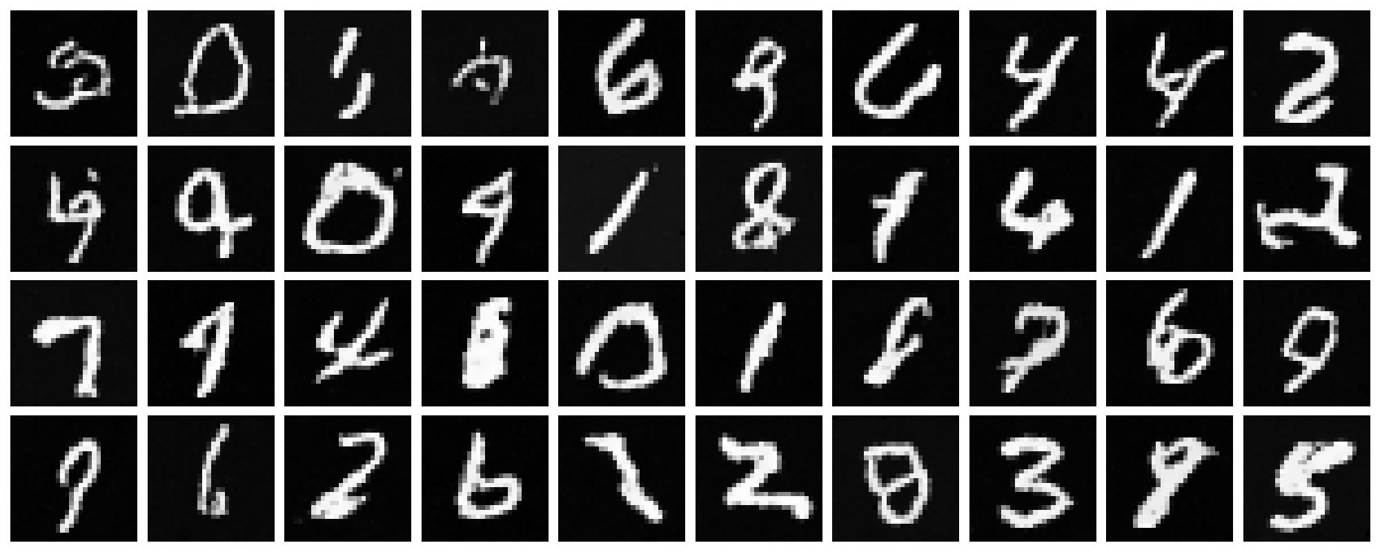
Sampling Results & Comparison
The last epoch's checkpoint was used to sample new images from the same pure noises as in B.2.3 for fair comparison. The sampled results are shown below (first image), alongside with those from B.2.3 (second image).
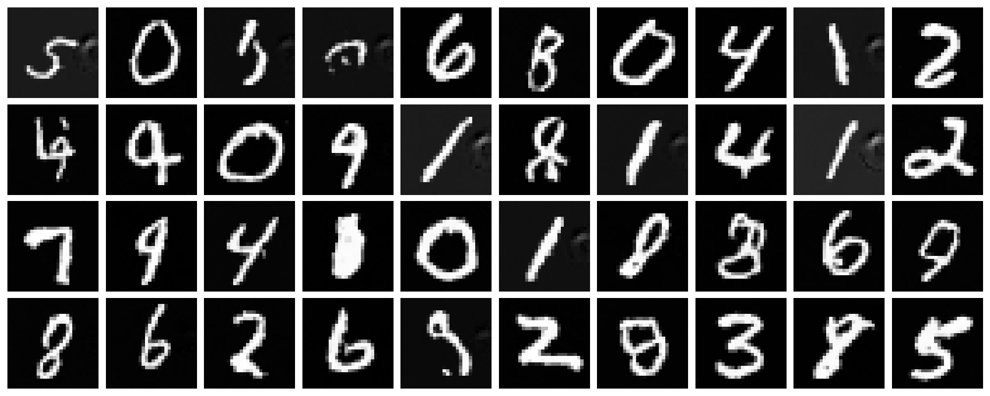
It can be observed that, even though the quality is still not as good as the class-conditioned model (due to the lack of class information and CFG), the generated digits are much clearer and distinguishable than before. Therefore, improving the model capacity is indeed helpful to enhance the generation quality when class conditioning is not available.